Krylov-space-based quasi-newton preconditioner for full-wavefield inversion
Akcelik , et al. November 17, 2
U.S. patent number 10,838,093 [Application Number 15/190,222] was granted by the patent office on 2020-11-17 for krylov-space-based quasi-newton preconditioner for full-wavefield inversion. This patent grant is currently assigned to ExxonMobil Upstream Research Company. The grantee listed for this patent is Volkan Akcelik, Huseyin Denli. Invention is credited to Volkan Akcelik, Huseyin Denli.


View All Diagrams
| United States Patent | 10,838,093 |
| Akcelik , et al. | November 17, 2020 |
Krylov-space-based quasi-newton preconditioner for full-wavefield inversion
Abstract
A method, including: storing, in a computer memory, seismic data acquired from a seismic survey of a subsurface region; and generating, with a computer, a final subsurface physical property model of the subsurface region by processing the seismic data with an iterative full wavefield inversion method, wherein the iterative full wavefield inversion method generates the final subsurface physical property model by iteratively applying a linear solver with a preconditioner that is generated from information from one or more previous iterations of the linear solver.
| Inventors: | Akcelik; Volkan (Spring, TX), Denli; Huseyin (Basking Ridge, NJ) | ||||||||||
|---|---|---|---|---|---|---|---|---|---|---|---|
| Applicant: |
|
||||||||||
| Assignee: | ExxonMobil Upstream Research
Company (Spring, TX) |
||||||||||
| Family ID: | 1000005185778 | ||||||||||
| Appl. No.: | 15/190,222 | ||||||||||
| Filed: | June 23, 2016 |
Prior Publication Data
| Document Identifier | Publication Date | |
|---|---|---|
| US 20170003409 A1 | Jan 5, 2017 | |
Related U.S. Patent Documents
| Application Number | Filing Date | Patent Number | Issue Date | ||
|---|---|---|---|---|---|
| 62188063 | Jul 2, 2015 | ||||
| Current U.S. Class: | 1/1 |
| Current CPC Class: | G01V 1/28 (20130101); G01V 1/306 (20130101); G01V 1/30 (20130101) |
| Current International Class: | G01V 1/30 (20060101); G01V 1/28 (20060101) |
References Cited [Referenced By]
U.S. Patent Documents
| 3812457 | May 1974 | Weller |
| 3864667 | February 1975 | Bahjat |
| 4159463 | June 1979 | Silverman |
| 4168485 | September 1979 | Payton et al. |
| 4545039 | October 1985 | Savit |
| 4562650 | January 1986 | Nagasawa et al. |
| 4575830 | March 1986 | Ingram et al. |
| 4594662 | June 1986 | Devaney |
| 4636957 | January 1987 | Vannier et al. |
| 4675851 | June 1987 | Savit et al. |
| 4686654 | August 1987 | Savit |
| 4707812 | November 1987 | Martinez |
| 4715020 | December 1987 | Landrum, Jr. |
| 4766574 | August 1988 | Whitmore et al. |
| 4780856 | October 1988 | Becquey |
| 4823326 | April 1989 | Ward |
| 4924390 | May 1990 | Parsons et al. |
| 4953657 | September 1990 | Edington |
| 4969129 | November 1990 | Currie |
| 4982374 | January 1991 | Edington et al. |
| 5260911 | November 1993 | Mason et al. |
| 5469062 | November 1995 | Meyer, Jr. |
| 5583825 | December 1996 | Carrazzone et al. |
| 5677893 | October 1997 | de Hoop et al. |
| 5715213 | February 1998 | Allen |
| 5717655 | February 1998 | Beasley |
| 5719821 | February 1998 | Sallas et al. |
| 5721710 | February 1998 | Sallas et al. |
| 5790473 | August 1998 | Allen |
| 5798982 | August 1998 | He et al. |
| 5822269 | October 1998 | Allen |
| 5838634 | November 1998 | Jones et al. |
| 5852588 | December 1998 | de Hoop et al. |
| 5878372 | March 1999 | Tabarovsky et al. |
| 5920838 | July 1999 | Norris et al. |
| 5924049 | July 1999 | Beasley et al. |
| 5999488 | December 1999 | Smith |
| 5999489 | December 1999 | Lazaratos |
| 6014342 | January 2000 | Lazaratos |
| 6021094 | February 2000 | Ober et al. |
| 6028818 | February 2000 | Jeffryes |
| 6058073 | May 2000 | Verwest |
| 6125330 | September 2000 | Robertson et al. |
| 6219621 | April 2001 | Hornbostel |
| 6225803 | May 2001 | Chen |
| 6311133 | October 2001 | Lailly et al. |
| 6317695 | November 2001 | Zhou et al. |
| 6327537 | December 2001 | Ikelle |
| 6374201 | April 2002 | Grizon et al. |
| 6381543 | April 2002 | Guerillot et al. |
| 6388947 | May 2002 | Washbourne et al. |
| 6480790 | November 2002 | Calvert et al. |
| 6522973 | February 2003 | Tonellot et al. |
| 6545944 | April 2003 | de Kok |
| 6549854 | April 2003 | Malinverno et al. |
| 6574564 | June 2003 | Lailly et al. |
| 6593746 | July 2003 | Stolarczyk |
| 6662147 | December 2003 | Fournier et al. |
| 6665615 | December 2003 | Van Riel et al. |
| 6687619 | February 2004 | Moerig et al. |
| 6687659 | February 2004 | Shen |
| 6704245 | March 2004 | Becquey |
| 6714867 | March 2004 | Meunier |
| 6735527 | May 2004 | Levin |
| 6754590 | June 2004 | Moldoveanu |
| 6766256 | July 2004 | Jeffryes |
| 6826486 | November 2004 | Malinverno |
| 6836448 | December 2004 | Robertsson et al. |
| 6842701 | January 2005 | Moerig et al. |
| 6859734 | February 2005 | Bednar |
| 6865487 | March 2005 | Charron |
| 6865488 | March 2005 | Moerig et al. |
| 6876928 | April 2005 | Van Riel et al. |
| 6882938 | April 2005 | Vaage et al. |
| 6882958 | April 2005 | Schmidt et al. |
| 6901333 | May 2005 | Van Riel et al. |
| 6903999 | June 2005 | Curtis et al. |
| 6905916 | June 2005 | Bartsch et al. |
| 6906981 | June 2005 | Vaage |
| 6927698 | August 2005 | Stolarczyk |
| 6944546 | September 2005 | Xiao et al. |
| 6947843 | September 2005 | Fisher et al. |
| 6970397 | November 2005 | Castagna et al. |
| 6977866 | December 2005 | Huffman |
| 6999880 | February 2006 | Lee |
| 7046581 | May 2006 | Calvert |
| 7050356 | May 2006 | Jeffryes |
| 7069149 | June 2006 | Goff et al. |
| 7027927 | July 2006 | Routh et al. |
| 7072767 | July 2006 | Routh et al. |
| 7092823 | August 2006 | Lailly et al. |
| 7110900 | September 2006 | Adler et al. |
| 7184367 | February 2007 | Yin |
| 7230879 | June 2007 | Herkenoff et al. |
| 7271747 | September 2007 | Baraniuk et al. |
| 7330799 | February 2008 | Lefebvre et al. |
| 7337069 | February 2008 | Masson et al. |
| 7373251 | May 2008 | Hamman et al. |
| 7373252 | May 2008 | Sherrill et al. |
| 7376046 | May 2008 | Jeffryes |
| 7376539 | May 2008 | Lecomte |
| 7400978 | July 2008 | Langlais et al. |
| 7436734 | October 2008 | Krohn |
| 7480206 | January 2009 | Hill |
| 7584056 | September 2009 | Koren |
| 7599798 | October 2009 | Beasley et al. |
| 7602670 | October 2009 | Jeffryes |
| 7616523 | November 2009 | Tabti et al. |
| 7620534 | November 2009 | Pita et al. |
| 7620536 | November 2009 | Chow |
| 7646924 | January 2010 | Donoho |
| 7672194 | March 2010 | Jeffryes |
| 7672824 | March 2010 | Dutta et al. |
| 7675815 | March 2010 | Saenger et al. |
| 7679990 | March 2010 | Herkenhoff et al. |
| 7684281 | March 2010 | Vaage et al. |
| 7710821 | May 2010 | Robertsson et al. |
| 7715985 | May 2010 | Van Manen et al. |
| 7715986 | May 2010 | Nemeth et al. |
| 7725266 | May 2010 | Sirgue et al. |
| 7791980 | September 2010 | Robertsson et al. |
| 7835072 | November 2010 | Izumi |
| 7840625 | November 2010 | Candes et al. |
| 7940601 | May 2011 | Ghosh |
| 8121823 | February 2012 | Krebs et al. |
| 8190405 | May 2012 | Appleyard |
| 8248886 | August 2012 | Neelamani et al. |
| 8428925 | April 2013 | Krebs et al. |
| 8437998 | May 2013 | Routh et al. |
| 8547794 | October 2013 | Gulati et al. |
| 8688381 | April 2014 | Routh et al. |
| 8781748 | July 2014 | Laddoch et al. |
| 9601109 | March 2017 | Horesh |
| 2002/0049540 | April 2002 | Beve et al. |
| 2002/0099504 | July 2002 | Cross et al. |
| 2002/0120429 | August 2002 | Ortoleva |
| 2002/0183980 | December 2002 | Guillaume |
| 2004/0199330 | October 2004 | Routh et al. |
| 2004/0225438 | November 2004 | Okoniewski et al. |
| 2006/0235666 | October 2006 | Assa et al. |
| 2007/0036030 | February 2007 | Baumel et al. |
| 2007/0038691 | February 2007 | Candes et al. |
| 2007/0274155 | November 2007 | Ikelle |
| 2008/0175101 | July 2008 | Saenger et al. |
| 2008/0306692 | December 2008 | Singer et al. |
| 2009/0006054 | January 2009 | Song |
| 2009/0067041 | March 2009 | Krauklis et al. |
| 2009/0070042 | March 2009 | Birchwood et al. |
| 2009/0083006 | March 2009 | Mackie |
| 2009/0164186 | June 2009 | Haase et al. |
| 2009/0164756 | June 2009 | Dokken et al. |
| 2009/0187391 | July 2009 | Wendt et al. |
| 2009/0248308 | October 2009 | Luling |
| 2009/0254320 | October 2009 | Lovatini et al. |
| 2009/0259406 | October 2009 | Khadhraoui et al. |
| 2010/0008184 | January 2010 | Hegna et al. |
| 2010/0018718 | January 2010 | Krebs et al. |
| 2010/0039894 | February 2010 | Abma et al. |
| 2010/0054082 | March 2010 | McGarry et al. |
| 2010/0088035 | April 2010 | Etgen et al. |
| 2010/0103772 | April 2010 | Eick et al. |
| 2010/0118651 | May 2010 | Liu et al. |
| 2010/0142316 | June 2010 | Keers et al. |
| 2010/0161233 | June 2010 | Saenger et al. |
| 2010/0161234 | June 2010 | Saenger et al. |
| 2010/0185422 | July 2010 | Hoversten |
| 2010/0208554 | August 2010 | Chiu et al. |
| 2010/0212902 | August 2010 | Baumstein et al. |
| 2010/0246324 | September 2010 | Dragoset, Jr. et al. |
| 2010/0265797 | October 2010 | Robertsson et al. |
| 2010/0270026 | October 2010 | Lazaratos et al. |
| 2010/0286919 | November 2010 | Lee et al. |
| 2010/0299070 | November 2010 | Abma |
| 2011/0000678 | January 2011 | Krebs et al. |
| 2011/0040926 | February 2011 | Donderici et al. |
| 2011/0051553 | March 2011 | Scott et al. |
| 2011/0075516 | March 2011 | Xia et al. |
| 2011/0090760 | April 2011 | Rickett et al. |
| 2011/0131020 | June 2011 | Meng |
| 2011/0134722 | June 2011 | Virgilio et al. |
| 2011/0182141 | July 2011 | Zhamikov et al. |
| 2011/0182144 | July 2011 | Gray |
| 2011/0191032 | August 2011 | Moore |
| 2011/0194379 | August 2011 | Lee et al. |
| 2011/0222370 | September 2011 | Downton et al. |
| 2011/0227577 | September 2011 | Zhang et al. |
| 2011/0235464 | September 2011 | Brittan et al. |
| 2011/0238390 | September 2011 | Krebs et al. |
| 2011/0246140 | October 2011 | Abubakar et al. |
| 2011/0267921 | November 2011 | Mortel et al. |
| 2011/0267923 | November 2011 | Shin |
| 2011/0276320 | November 2011 | Krebs et al. |
| 2011/0288831 | November 2011 | Tan et al. |
| 2011/0299361 | December 2011 | Shin |
| 2011/0320180 | December 2011 | Ai-Saleh |
| 2012/0010862 | January 2012 | Costen |
| 2012/0014215 | January 2012 | Saenger et al. |
| 2012/0014216 | January 2012 | Saenger et al. |
| 2012/0051176 | March 2012 | Liu |
| 2012/0073824 | March 2012 | Routh |
| 2012/0073825 | March 2012 | Routh |
| 2012/0082344 | April 2012 | Donoho |
| 2012/0143506 | June 2012 | Routh et al. |
| 2012/0215506 | August 2012 | Rickett et al. |
| 2012/0218859 | August 2012 | Soubaras |
| 2012/0275264 | November 2012 | Kostov et al. |
| 2012/0275267 | November 2012 | Neelamani et al. |
| 2012/0290214 | November 2012 | Huo et al. |
| 2012/0314538 | December 2012 | Washbourne et al. |
| 2012/0316790 | December 2012 | Washbourne et al. |
| 2012/0316791 | December 2012 | Shah |
| 2012/0316844 | December 2012 | Shah et al. |
| 2013/0060539 | March 2013 | Baumstein |
| 2013/0081752 | April 2013 | Kurimura et al. |
| 2013/0238246 | September 2013 | Krebs et al. |
| 2013/0279290 | October 2013 | Poole |
| 2013/0282292 | October 2013 | Wang et al. |
| 2013/0311149 | November 2013 | Tang |
| 2013/0311151 | November 2013 | Plessix |
| 2014/0350861 | November 2014 | Wang et al. |
| 2014/0358504 | December 2014 | Baumstein et al. |
| 2014/0372043 | December 2014 | Hu et al. |
| 2015/0073755 | March 2015 | Tang et al. |
| 2016/0238729 | August 2016 | Warner |
| 2 796 631 | Nov 2011 | CA | |||
| 1 094 338 | Apr 2001 | EP | |||
| 1 746 443 | Jan 2007 | EP | |||
| 2 390 712 | Jan 2004 | GB | |||
| 2 391 665 | Feb 2004 | GB | |||
| WO 2006/037815 | Apr 2006 | WO | |||
| WO 2007/046711 | Apr 2007 | WO | |||
| WO 2008/042081 | Apr 2008 | WO | |||
| WO 2008/123920 | Oct 2008 | WO | |||
| WO 2009/067041 | May 2009 | WO | |||
| WO 2009/117174 | Sep 2009 | WO | |||
| WO 2010/085822 | Jul 2010 | WO | |||
| WO 2011/040926 | Apr 2011 | WO | |||
| WO 2011/091216 | Jul 2011 | WO | |||
| WO 2011/093945 | Aug 2011 | WO | |||
| WO 2012/024025 | Feb 2012 | WO | |||
| WO 2012/041834 | Apr 2012 | WO | |||
| WO 2012/083234 | Jun 2012 | WO | |||
| WO 2012/134621 | Oct 2012 | WO | |||
| WO 2012/170201 | Dec 2012 | WO | |||
| WO 2013/081752 | Jun 2013 | WO | |||
Other References
|
Nocedal, J. "Updating Quasi-Newton Matrices with Limited Storage" Mathematics of Computation, vol. 35, No. 151, pp. 773-782 (1980) (Year: 1980). cited by examiner . Nocedal, J. "Numerical Optimization" 2nd Ed. (2006) (Year: 2006). cited by examiner . U.S. Appl. No. 14/329,431, filed Jul. 11, 2014, Krohn et al. cited by applicant . U.S. Appl. No. 14/330,767, filed Jul. 14, 2014, Tang et al. cited by applicant . Akcelik, V., et al. (2006) "Parallel algorithms for PDE constrained optimization, in Parallel Processing for Scientific Computing", SIAM, 2006; Ch 16, pp. 291-322. cited by applicant . Knoll, D.A. and Keyes, D.E., (2004) "Jacobian-free Newton-Krylov Methods: A Survey of Approaches and Applications", Journal of Computational Physics 193, 357-397. cited by applicant . Krebs, J.R., et al. (2009) "Fast Full-wavefield Seismic Inversion Using Encoded Sources", Geophysics, 74, No. 6, pp. WCC177-WCC188. cited by applicant . Metivier, L. et al. (2013) "Full Waveform Inversion and Truncated Newton Method", SIAM J. Sci. Comput., 35(2), B401-6437. cited by applicant . Morales, J.L. and Nocedal, J. (2000) "Automatic Preconditioning by Limited Memory Quasi-Newton Updating", SIAM J. Optim, 10(4), 1079-1096. cited by applicant . Nocedal, J. and Wright, J. (2006) "Numerical Optimization", 2nd Edition, Springer; pp. I-Xii, 101-192. cited by applicant . Akcelik, V., et al. (2002) "Parallel Multiscale Gauss-Newton-Krylov Methods for Inverse Wave Propogation", Supercompuiting, ACM/IEEE 2002 Conference Nov. 16-22, 2002. cited by applicant . Metivier, L. et al. (2014) "Full Waveform Inversion and Truncated Newton Method: quantitative imaging of complex subsurface structures", Geophysical Prospecting, vol. 62, pp. 1353-1375. cited by applicant . Virieux, J. et al. (2009) "An overview of full-waveform inversion in exploration geophysics", Geophysics, vol. 74, No. 6.pp. WCC127-WCC152. cited by applicant. |
Primary Examiner: Hann; Jay
Attorney, Agent or Firm: ExxonMobil Upstream Research Company--Law Department
Parent Case Text
CROSS-REFERENCE TO RELATED APPLICATION
This application claims the benefit of U.S. Provisional Patent Application 62/188,063 filed Jul. 2, 2015 entitled KRYLOV-SPACE-BASED QUASI-NEWTON PRECONDITIONER FOR FULL WAVEFIELD INVERSION, the entirety of which is incorporated by reference herein.
Claims
The invention claimed is:
1. A method, comprising: storing, in a computer memory, seismic data acquired from a seismic survey of a subsurface region; generating, with a computer, a final subsurface physical property model of the subsurface region by processing the seismic data with an iterative full wavefield inversion method, wherein the iterative full wavefield inversion method includes a non-linear outer iteration process comprising a plurality of outer iterations, each of which updates physical property values m of the physical property model and a nested linear inner iteration process, wherein: (1) each iteration i of the plurality of non-linear outer iterations includes a nested linear inner iteration process for determining a search direction d.sub.i to be used in updating the physical property values m.sub.i of said non-linear outer iteration; and (2) each of the second and subsequent outer iterations of the plurality of non-linear outer iterations further includes applying a preconditioner to the nested linear inner iteration process of such respective second and subsequent non-linear outer iteration, wherein the preconditioner at such non-linear outer iteration i+1 is generated based at least in part upon the nested linear inner iteration process of the immediately previous outer iteration i and wherein the preconditioner is generated using vectors {.gamma..sup.l, H.sub.i.gamma..sup.l} solved for in the nested inner iteration process, where .gamma..sup.l is the search direction for the linear system and where H.sub.i.gamma..sup.l is the product of the vector .gamma..sup.l with a Hessian operator H.sub.i; and creating, with a process, an image of the subsurface region from the final subsurface physical property model.
2. The method of claim 1, comprising using a Krylov-space method as a linear solver for the nested inner iteration processes.
3. The method of claim 1, comprising using a conjugate gradient method as a linear solver for the nested inner iteration processes.
4. The method of claim 2, wherein each preconditioner is generated based on the nested inner iteration process of the immediately previous outer iteration using a limited-memory Broyden-Fletcher-Goldfarb-Shanno (BFGS) method.
5. The method of claim 2, wherein each preconditioner is generated based on the nested inner iteration process of the immediately previous outer iteration using a quasi-Newton method.
6. The method of claim 1, wherein the preconditioner of each of the second and subsequent outer iterations is a variable preconditioner such that the preconditioner can change when solving a linear system, and the preconditioner is generated based on the nested iteration process of the then-current outer iteration in addition to the nested inner iteration process of the immediately previous outer iteration.
7. The method of claim 1, further comprising managing hydrocarbons based on the final subsurface physical property model of the subsurface region.
8. The method of claim 1, further comprising: using the final subsurface physical property model in interpreting a subsurface region for hydrocarbon exploration or production.
9. The method of claim 1, further comprising drilling for hydrocarbons at a location determined using the final subsurface physical property model of the subsurface region.
10. The method of claim 1, wherein a generalized minimal residual method is used as a linear solver for the nested inner iteration processes.
Description
FIELD OF THE INVENTION
Exemplary embodiments described herein pertain generally to the field of geophysical prospecting, and more particularly to geophysical data processing. An exemplary embodiment can increase the speed of convergence of full wavefield inversion (FWI).
BACKGROUND
This section is intended to introduce various aspects of the art, which may be associated with exemplary embodiments of the present technological advancement. This discussion is believed to assist in providing a framework to facilitate a better understanding of particular aspects of the present technological advancement. Accordingly, it should be understood that this section should be read in this light, and not necessarily as admissions of prior art.
Seismic inversion is a process of extracting subsurface information from the data measured at the surface of the earth acquired during a seismic survey. In a typical seismic survey, seismic waves are generated by a source positioned at desired locations. As the source generated wave propagates through the subsurface and travels back to the receiver locations where it is recorded.
Full waveform inversion (FWI) is a seismic processing method which can potentially exploit the full seismic record including events that are treated as "noise" by standard seismic processing algorithms. FWI iteratively minimizes an objective function based on a comparison of a simulated and measured seismic records. Even with today's available high-performance computing resources, one of the biggest challenges to FWI is still the computational cost. Nevertheless, the benefit of inferring a detailed representation of the subsurface using this method is expected to outweigh this cost, and development of new algorithms and workflows that lead to faster turnaround time is a key step towards making this technology feasible for field-scale applications, allowing users to solve larger scale problems faster. The computationally most intensive component of FWI is the simulations of the forward and adjoint wavefields. The number of total forward and adjoint simulations is proportional to the number of iterations, which is typically on the order of hundreds to thousands. Any method reducing number of FWI iterations will reduce to number of forward and adjoint simulation calls and the computational run time.
The crux of any FWI algorithm can be described as follows: using a given starting subsurface physical property model, synthetic seismic data are generated, i.e. modeled or simulated, by solving the wave equation using a numerical scheme (e.g., finite-difference, finite-element, spectral element, and etc.) which typically divides the model domain into a set of nonoverlapping cells (also referred as elements or blocks). The term velocity model or geophysical property model as used herein refers to an array of numbers, where each number, which may also be called a model parameter, is a value of velocity or another geophysical property in a cell. The synthetic seismic data are compared with the field seismic data and using a norm, an error or objective function is calculated. Using this objective function and an optimization algorithm, a modified subsurface model is generated which is used to simulate a new set of synthetic seismic data. This new set of synthetic seismic data is compared with the field data to generate a new objective function. This process is repeated until the optimization algorithm satisfactorily minimizes the objective function and the final subsurface model is generated. A global or local optimization method is used to minimize the objective function and to update the subsurface model. Further details regarding FWI can be found in U.S. Patent Publication 2011/0194379 to Lee et al., the entire contents of which are hereby incorporated by reference.
Common FWI methods iteratively minimize the objective function which is subject to the wavefield propagation--the physics of the problem. A (nonlinear) iteration i of FWI involves the following two steps: (1) compute a search direction for the current model m.sub.i, d(m.sub.i); and (2) search for an update to the current model which is a perturbation along the search direction and that reduces the objective function. The FWI processing starts from a given starting model m.sub.0 provided by the user. FWI algorithms iteratively improve this starting model using an optimization technique, m.sub.i+1=m.sub.i+.alpha..sub.id.sub.i, (1) where .alpha..sub.i is a scalar parameter, d.sub.i is the search direction and i is the nonlinear iteration number. The search direction is chosen along a globalization strategy [1,2]. For the second-order optimization methods, the search direction is obtained by solving H.sub.id.sub.i=-g.sub.i, (2) where H.sub.i can be Newton's Hessian or Gauss-Newton's Hessian. For the large scale optimization problems, the Hessian is both prohibitively large to store and compute explicitly. Instead, an approximate inverse Hessian H.sub.i.sup.-1 is used to calculate the search direction. There are several choices for this approximation, such as (i) quasi-Newton methods and (ii) truncated Newton's or Gauss-Newton methods (note that "(Gauss)-Newton" is used herein to refer to both Newton and Gauss-Newton methods).
SUMMARY
In an exemplary embodiment, a method can include: storing, in a computer memory, seismic data acquired from a seismic survey of a subsurface region; and generating, with a computer, a final subsurface physical property model of the subsurface region by processing the seismic data with an iterative full wavefield inversion method, wherein the iterative full wavefield inversion method generates the final subsurface physical property model by iteratively applying a linear solver with a preconditioner that is generated from information from one or more previous iterations of the linear solver.
In an exemplary embodiment, the linear solver is a Krylov-space method.
In an exemplary embodiment, the linear solver is a conjugate gradient method.
In an exemplary embodiment, the method can further include generating the preconditioner with a limited-memory Broyden-Fletcher-Goldfarb-Shanno (BFGS) method.
In an exemplary embodiment, the method can further include generating the preconditioner with a quasi-Newton method.
In an exemplary embodiment, the method can further include: storing, in a computer memory, a change in an optimization parameter of the full wavefield inversion method and a change in a gradient of a cost function used in the full wavefield inversion method for each of a plurality of iterations of the linear solver; generating the preconditioner based on the change in the optimization parameter and the change in the gradient of the cost function from each of the plurality of iterations of the linear solver; and applying the preconditioner to a subsequent iteration of the linear solver, relative to the plurality of iterations.
In an exemplary embodiment, the preconditioner is a fixed preconditioner, and the preconditioner does not change when solving a linear system and it is only based on changes in the optimization parameter and changes in the gradient of the cost function from previous iterations of the linear solver.
In an exemplary embodiment, the preconditioner is a variable preconditioner, and the preconditioner can change when solving a linear system, and is based on changes in the optimization parameter and changes in the gradient of the cost function from previous iterations of the linear solver and a current linear iteration of the linear solver.
In an exemplary embodiment, the linear solver is non-flexible.
In an exemplary embodiment, the linear solver is flexible.
In an exemplary embodiment, the change in the optimization parameter for a standard quasi-Newton algorithm is replaced with a change in a search direction of a linear system.
In an exemplary embodiment, the change in the gradient for the standard quasi-Newton algorithm is replaced with a change in a residual of the linear solver.
In an exemplary embodiment, the optimization parameter is the search direction and the gradient is a residual of a linear system.
In an exemplary embodiment, the linear solver is a Krylov-space method.
In an exemplary embodiment, the method can further include managing hydrocarbons based on the final subsurface physical property model of the subsurface region.
In an exemplary embodiment, the method can further include: creating, with a processor, an image of the subsurface region from the final subsurface physical property model.
In an exemplary embodiment, the method can further include: using the final subsurface physical property model in interpreting a subsurface region for hydrocarbon exploration or production.
In an exemplary embodiment, the method can further include drilling for hydrocarbons at a location determined using the final subsurface physical property model of the subsurface region.
In an exemplary embodiment, the linear solver is a generalized minimal residual method.
BRIEF DESCRIPTION OF THE DRAWINGS
While the present disclosure is susceptible to various modifications and alternative forms, specific example embodiments thereof have been shown in the drawings and are herein described in detail. It should be understood, however, that the description herein of specific example embodiments is not intended to limit the disclosure to the particular forms disclosed herein, but on the contrary, this disclosure is to cover all modifications and equivalents as defined by the appended claims. It should also be understood that the drawings are not necessarily to scale, emphasis instead being placed upon clearly illustrating principles of exemplary embodiments of the present invention. Moreover, certain dimensions may be exaggerated to help visually convey such principles.
FIG. 1 illustrates the linear and nonlinear iterative methods that are included in the present technological advancement.
FIG. 2 illustrates an exemplary method embodying the present technological advancement.
FIG. 3 describes an exemplary application of the present technological advancement.
DESCRIPTION OF THE INVENTION
While the present disclosure is susceptible to various modifications and alternative forms, specific example embodiments thereof have been shown in the drawings and are herein described in detail. It should be understood, however, that the description herein of specific example embodiments is not intended to limit the disclosure to the particular forms disclosed herein, but on the contrary, this disclosure is to cover all modifications and equivalents as defined by the appended claims. It should also be understood that the drawings are not necessarily to scale, emphasis instead being placed upon clearly illustrating principles of exemplary embodiments of the present invention. Moreover, certain dimensions may be exaggerated to help visually convey such principles.
The present technological advancement can increase the speed for convergence of FWI by several factors when second order methods are used as the optimization technique. The present technological advancement can uniquely combine two known optimization techniques: the quasi-Newton methods (such as L-BFGS) (first method) and the truncated Newton-or Gauss-Newton)-method (second method). In the present technological advancement, the second method can be used as an optimization algorithm and the first method can be used to speed up the convergence of the second method as a preconditioner.
Quasi-Newton Methods
Quasi-Newton methods replace H.sub.i.sup.-1 with its approximation in equation (2) when solving for d. These methods approximate the inverse Hessian operator (H) using gradient and model parameter changes throughout nonlinear iteration (this can be contrasted with (Gauss) Newton's method, which does not approximate the Hessian, but (approximately) solves Equation (2)).
Not all quasi-Newton methods are directly applicable to FWI problems due to its large-scale nature. However, quasi-Newton methods are modified and extended in several ways to make them suitable for large-scale optimization problems. The members of the quasi-Newton methods suitable for large scale optimization problems are so called limited-memory quasi-Newton methods. The limited-memory BFGS (Broyden-Fletcher-Goldfarb-Shanno) (L-BFGS) algorithm is the most common member suitable for FWI, as it is robust and computationally inexpensive and easy to implement [2]. All the preconditioner approaches introduced in the rest of the discussion will be based on the L-BFGS algorithm. However, the present technological advancement is not limited to the use of the L-BFGS algorithm; and other quasi-Newton algorithms such as limited memory SR1 method could also be used [2].
The inverse Hessian approximation H.sub.i+1.sup.-1 will be dense, so the cost of storing and manipulating it is computationally prohibitive for an FWI problem. To circumvent this problem, in limited memory BFGS approximation, {s.sub.i,y.sub.i} pairs are used to approximate the action of H.sub.i+1.sup.-1 to a given vector. The vector pairs {s.sub.i,y.sub.i} are defined as s.sub.i=m.sub.i+1-m.sub.i, and (3) y.sub.i=g.sub.i+1-g.sub.i. (4)
In other words, vector s.sub.i is the change in optimization parameter and vector y.sub.i is the change in the gradient g.sub.i, at nonlinear iteration i.
The resulting recursive algorithm computes the application of the approximate inverse Hessian on a vector q by the L-BFGS approach using m pairs of {s.sub.i,y.sub.i} is given in Algorithm (1) below. Note that given vector q and m vector pairs {s.sub.i,y.sub.i}, the algorithm returns the vector p, which is multiplication of the approximate inverse Hessian with vector q.
TABLE-US-00001 Algorithm 1: Two-loop L-BFGS algorithm [2] FOR (k = m, m - 1, ... ,1) (m is the total number of pairs and k is the iterator for the loop) .alpha..times..times. ##EQU00001## q = q - .alpha..sub.ky.sub.k END FOR p = (H.sub.i.sup.0).sup.-1q FOR (k = 1,2, ... , m) .beta..times..times. ##EQU00002## p = p + (.alpha..sub.k - .beta.)s.sub.k END FOR RETURN p
To complete the given L-BFGS algorithm (1), an initial estimate (H.sub.i.sup.0).sup.-1 needs to be provided to the algorithm. A method for choosing (H.sub.i.sup.0).sup.-1 that has proven to be effective in practice is to set
.times..times..times. ##EQU00003## where the multiplier in front of identity matrix (I) is the scaling factor that attempts to estimate the size of the true Hessian matrix along the most recent search direction. The choice of scaling factor is important to ensure that the initial Hessian approximation is accurately scaled. Alternatively, the initial estimate (H.sub.i.sup.0).sup.-1 can be set to an available geophysics based preconditioner (such as U.S. Patent Publication No. 2015/0073755, the entirety of which is incorporated by reference). This mechanism enables different types of preconditioners to be combined with the present technological advancement.
Truncated (Gauss)-Newton Method
Another approach for solving the (Gauss)-Newton system (2) is to use an iterative method. In contrast to the Quasi-Newton method, this approach uses the Hessian operator (or its approximation as in Gauss-Newton method) directly. However, due to difficulty of storing and explicitly computing the Hessian operator, one can only employ an iterative method to solve (2) since these methods do not explicitly require the Hessian operator in (2) but rather they require application of the Hessian operator to a given vector. A preferred approach is to use one of the so-called Krylov space methods. A Krylov space method for solving a linear system Ax=b is an iterative method starting from some initial approximation x.sub.0 and the corresponding residual r.sub.0=b-Ax.sub.0, and iterating until the process possibly finds the exact solution or a stopping criteria is satisfied. These methods only require application of the Hessian operator to a given vector. For an FWI, application of Hessian on a vector can require computing at least one forward and one adjoint simulations of the wavefields. The linear iterations usually terminate using inner convergence criteria to improve speed of the nonlinear convergence of FWI[1, 2, 6]. The following discussion will utilize the conjugate gradient method as a non-limiting example of a Krylov space method.
After the search direction is computed by approximately solving (2) with an iterative linear Krylov-space solver (such as the conjugate gradient method), the FWI model is updated using a line search strategy. This procedure is repeated till convergence (see FIG. 1). The linear iterations for solving the system (2) with the conjugate gradient method are referred to as inner iterations 101, and the nonlinear iterations for updating the optimization parameter m.sub.i are referred to as outer iterations 103, and the relationship between the two are depicted in FIG. 1.
The accompanying Appendix provides additional information regarding implementation of the conjugate gradient method.
Preconditioning
When using the truncated (Gauss)-Newton method, the performance of linear solvers used to solve (2) can be improved by using a preconditioner. In this case, instead of solving equation (2), the following system is solved with the Krylov space methods B.sub.i.sup.-1H.sub.id.sub.i=-B.sub.i.sup.-1g.sub.i, (6) where B.sub.i.sup.-1 is the preconditioner to equation system (2) which is typically an approximation to the numerical inverse of the Hessian for optimization problems. One of the roles of the preconditioner is to reduce the condition number of the Hessian, so that equation system (6) can be solved more efficiently with less linear iterations. Note that, in (6) the preconditioner is applied from the left side of the operator H.sub.i. There are other alternatives applications of the preconditioner, and the present technological advancement is not limited to the example provided here. (See Appendix, [2,6]).
Exemplary Embodiments
In following non-limiting exemplary embodiments of the present technological advancement, three methods are combined in a unique way: (i) Quasi-Newton method, (ii) truncated (Gauss)-Newton method and (iii) preconditioning. These exemplary embodiments use the truncated (Gauss)-Newton method as the optimization algorithm. In addition, the quasi-Newton approximation of the inverse Hessian is used as a preconditioner to the (Gauss)-Newton system. In other words, Algorithm 1 is used as a preconditioner when solving the system (2) using a Krylov-space method. To create the preconditioner of Algorithm 1, either information from the outer nonlinear iterations 103 or inner linear iterations 101 can be used to construct the preconditioner [1]. The main difference in these approaches (and one example of where the present technological advancement differentiates itself from the state-of-the art [1]) is the way the vector pairs {s.sub.i,y.sub.i} are created and used in the application of Algorithm 1 by the present technological advancement.
The state-of-the-art quasi-Newton preconditioning approach essentially approximates the inverse Hessian using the information captured from the outer iterations. The present technological advancement, on the contrary, introduces a quasi-Newton preconditioner which approximates the inverse Hessian using the history of inner iterations 101. The present technological advancement may include the use of any additional preconditioner to Algorithm 1 as a starting initial estimate of equation (5) for the iterative process. The present technological advancement significantly improves the convergence speed of FWI relative to the state-of-the-art preconditioning methods with an additional negligible computational cost.
First, it is observed that the solution of equation (2) via an iterative Krylov space method is equivalent to minimization of the following unconstrained quadratic optimization problem of the form
.times..times..function..times..times..times..times. ##EQU00004##
It is noted that solving (2) with a Krylov subspace method, such as the conjugate gradient method, is equivalent to minimizing an objective function in the form of (7). This idea is combined with the quasi-Newton method to create a preconditioner for the truncated Newton (or truncated Gauss-Newton) method.
In solving (2) with a Krylov-subspace method, the optimization parameter is the search direction d.sub.i and the gradient is equivalent to residual of the linear system (2). At a given inner linear iteration l, the gradient of the objective function (7) (also the residual of linear system (2)) is r.sup.l=H.sub.id.sub.i.sup.l+g.sub.i. (8).
In a given linear iteration of the conjugate gradient method, the solution of (2) is updated with d.sub.i.sup.l+1=d.sub.i.sup.l+.mu..sup.l.gamma..sup.l. (9).
And the residual (gradient) is updated with r.sup.l+1=r.sup.l+.mu..sup.lH.sub.i.gamma..sup.l, (10) where .mu..sup.l is the step length and .gamma..sup.l is the search direction for the linear system (see [2, Appendix] for details).
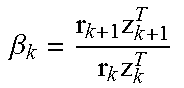
The present technological advancement constructs the quasi-Newton preconditioner with the information captured from this inner optimization, {s.sub.i,y.sub.i} pairs in equation (7). Using equation (3) and (4) along with (8) and (9) we get y.sup.l=r.sup.l+1-r.sup.l=.mu..sup.lH.sub.i.gamma..sup.l, and (11) s.sup.l=d.sub.i.sup.l+1-d.sub.i.sup.l=.mu..sup.l.gamma..sup.l. (12) In contrast, the quasi-Newton method uses outer nonlinear iterations to create {s.sub.l,y.sub.l} pairs.
Noting that scaling factor .mu..sup.l in (11) and (12) can be omitted because it cancels out in the application of the preconditioner, leading to s.sup.l=.gamma..sup.l and y.sup.l=H.sub.i.gamma..sup.l. (13)
To generate the preconditioner, the vectors in (13) are substituted into Algorithm 1, wherein the output is the multiplication of the approximate inverse Hessian with vector q, wherein this vector q can be the residual vector r in the preconditioned conjugate gradient method (see Appendix).
These choices of vectors (13) and their use, for example, are ways in which the present technological advancement distinguishes over the conventional techniques. In other words, on using inner iterations 101 of Krylov-space method (conjugate gradient method) as a linear solver, it is recognized that: "the change in the residual of inner iterations" plays the same role as "change in the gradient of outer iterations", and "the change in the solution of the linear system" plays the same role as "the change in the solution of the outer optimization system".
FIG. 1 is a depiction of the outer and inner iterations that are part of the truncated (Gauss)-Newton method, and how they relate to generating an updated physical properties subsurface model. The linear or inner iterations 101.sub.i are repeated for equations (7)-(12) until a predetermined stopping criteria is reached, at which point d.sub.i is determined. As part of these iterations, L {s.sub.l,y.sub.l} pairs are generated in linear iterations 101.sub.i, stored, and used to create the preconditioner for use in subsequent iterations. d.sub.i, the output of the first linear iteration 101.sub.i in FIG. 1, is used to update the model m at the outer iteration 103.sub.i, which is repeated for the subsequent outer iterations. The outer 103 and inner 101 iterations are repeated until the updated model converges or some other predetermined stopping criteria is satisfied.
FIG. 2 is a flow chart for an exemplary method of implementing the present technological advancement. The exemplary method of FIG. 2 builds on the truncated (Gauss)-Newton method of FIG. 1 by combining it with quasi-Newton methods and preconditioning.
In step 201, in the first non-linear iteration 103i, equation (2) is solved using the conjugate gradient method, without preconditioning, by performing several linear iterations 101.sub.i of the conjugate gradient method. Since (s.sub.k, y.sub.k) pairs are not available for the first iteration, the preconditioner of the present technological advancement is not used in the first nonlinear iteration. However, it is also possible to use another preconditioner when performing step 201.
In step 203, in the first nonlinear iteration 103.sub.i, when solving equation (2), vectors .gamma..sup.l, and its product with the Hessian operator H.sub.i.gamma..sup.l are stored in computer memory. Effectively, the right most terms in equations (9) and (10) can be stored for each iteration 1. As noted above, the scaling factor will cancel out and effectively it does not matter whether the scaling factor is stored along with vectors .gamma..sup.l and its product with the Hessian operator H.sub.i.gamma..sup.l.
In step 205, the model is updated in outer iteration 103.sub.i. The output of the inner iterations 101.sub.i is d.sub.i, which is used to update the model in the outer iteration 103.sub.i.
In step 207, in the second nonlinear iteration 103.sub.i+1, the stored pairs of {.gamma..sup.l, H.sub.i.gamma..sup.l} from the previous nonlinear iteration 103.sub.i are used to construct quasi-Newton "inverse Hessian mat-vec (matrix-free) operator" (Algorithm 1). This operator is used for preconditioning the conjugate gradient algorithm as given in equation (6). Only the pairs stored in the previous outer iteration(s) are used in the preconditioner application when a non-flexible conjugate gradient method is used. However, flexible version of the conjugate gradient method can also be used with the present technological advancement. The flexible version allows for a variable preconditioner within inner iterations 101. In this case, a slight modification in the application of the preconditioner is possible. Accordingly, the flexible version of the conjugate gradient method can use all pairs of {.gamma..sup.l, H.sub.i.gamma..sup.l} vectors (i.e., those from the previous nonlinear iteration 103.sub.i and those generated during the current nonlinear iteration 103.sub.i+1). Further details of this flexible preconditioner approach are included in the Appendix.
The L-BFGS preconditioner requires a starting inverse Hessian, which is above approximated by scaled identity (5). The correct scaling can be crucial for the performance of the preconditioner. When Algorithm 1 is used as part of the present technological advancement to generate the preconditioner, the state-of-the-art preconditioner (5) constructed from the information at the outer iterations can be used as a starting inverse Hessian. Thus, the present technological advancement can combine information obtained from both the outer and inner iterations.
Provided that H.sub.i in (2) is positive definite for a Gauss-Newton system, it can be shown that the resultant algorithm produces a positive definite operator, and guarantees a decent direction and robust algorithm. If one uses a truncated Newton's method, additional care must be taken to preserve positive definiteness [2].
In step 209, in the second linear iterations 101.sub.i+1, the process continues to store the pairs of {.gamma..sup.l, H.sub.i.gamma..sup.l} vectors generated from the current iteration (i+1) during the solving of equation (6) using the conjugate gradient method.
In step 211, the model is updated in outer iteration 103.sub.i+1. The output of the inner iterations 101.sub.i+1 is d.sub.i+1, which is used to update the model in the outer iteration 103.sub.i+1.
In step 213, it is determined whether convergence criteria or other predetermined stopping criteria has been reached for the updated physical property model. If not, the process returns to step 207 for another iteration. Iterations can continue until the convergence or stopping criteria is satisfied.
When the convergence or stopping criteria is satisfied, the process proceeds to step 215, in which a final physical property subsurface model is generated.
In step 217, the final physical property subsurface model can be used to manage hydrocarbon exploration. As used herein, hydrocarbon management includes hydrocarbon extraction, hydrocarbon production, hydrocarbon exploration, identifying potential hydrocarbon resources, identifying well locations, determining well injection and/or extraction rates, identifying reservoir connectivity, acquiring, disposing of and/or abandoning hydrocarbon resources, reviewing prior hydrocarbon management decisions, and any other hydrocarbon-related acts or activities.
The preconditioner of the present technological advancement can be used along with alternative iterative methods. The above examples use the conjugate gradient method as the linear solver. The conjugate gradient method can be replaced with another iterative method, such as the generalized minimal residual method (GMRES). To be applicable to FWI, such alternative methods need to be iterative like the conjugate gradient method.
Construction of the preconditioner of the present technological advancement is not limited to Algorithm 1. Other alternative iterative methods such as limited memory SR1 can be used. The update vectors of Algorithm 1 are the change in the residual at each iteration and the change of the iteration of the linear solver.
FIG. 3 illustrates a comparison between the present technological advancement and conventional technology. The comparison is based on the data synthetically generated using a geologically appropriate model, and uses a state-of-the-art truncated-Gauss-Newton method as the baseline algorithm. FIG. 3 displays the convergence speed-up with the present technological advancement when it is used for a sequential-source [5] FWI problem constructing-the model.
In all practical applications, the present technological advancement must be used in conjunction with a computer, programmed in accordance with the disclosures herein. Preferably, in order to efficiently perform FWI, the computer is a high performance computer (HPC), known as to those skilled in the art. Such high performance computers typically involve clusters of nodes, each node having multiple CPU's and computer memory that allow parallel computation. The models may be visualized and edited using any interactive visualization programs and associated hardware, such as monitors and projectors. The architecture of system may vary and may be composed of any number of suitable hardware structures capable of executing logical operations and displaying the output according to the present technological advancement. Those of ordinary skill in the art are aware of suitable supercomputers available from Cray or IBM.
The present techniques may be susceptible to various modifications and alternative forms, and the examples discussed above have been shown only by way of example. However, the present techniques are not intended to be limited to the particular examples disclosed herein. Indeed, the present techniques include all alternatives, modifications, and equivalents falling within the spirit and scope of the appended claims.
REFERENCES
The following references are each incorporated by the reference in their entirety: [1] L. Metivier, R. Brossier, J. Virieux, and S. Operto, "Full Waveform Inversion and Truncated Newton Method", SIAM J. Sci. Comput., 35(2), B401-B437; [2] J. Nocedal and J. Wright, "Numerical Optimization", 2nd Edition, Springer; [3] V. Akcelik, G. Biros, O. Ghattas, J. Hill, D. Keyes, and B. van Bloemen Waanders, "Parallel algorithms for PDE constrained optimization, in Parallel Processing for Scientific Computing", SIAM, 2006; [4] J. L. Morales and J. Nocedal, "Automatic Preconditioning by Limited Memory Quasi-Newton Updating", SIAM J. Optim, 10(4), 1079-1096; [5] J. R. Krebs, J. E. Anderson, D. Hinkley, R. Neelamani, S. Lee, A. Baumstein and M. D. Lacasse, "Fast Full-wavefield Seismic Inversion Using Encoded Sources", Geophysics, 74; and [6] D. A. Knoll and D. E. Keyes, "Jacobian-free Newton-Krylov Methods: A Survey of Approaches and Applications", SIAM J. Sci. Comp. 24:183-200, 2002.
APPENDIX
The conjugate gradient method is an algorithm for finding the numerical solution of symmteric and positive-definite systems of linear equations. The conjugate gradient method is often implemented as an iterative algorithm, applicable to sparse systems that are too large to be handled by a direct implementation or other direct methods such as the Cholesky decomposition. Large sparse systems often arise when numerically solving partial differential equations or optimization problems. The conjugate gradient method can also be used to solve unconstrained optimization problems such as least squares minimization problem.
Description of the Method
Suppose solving the following system of linear equations Ax=b, (A1) for the vector x, where b is the known vector, and A is the known n-by-n matrix which is symmetric (i.e., A.sup.T=A), positive definite (x.sup.TAx>0 for all non-zero vectors x in ), and real. The unique solution of this system is given by x*.
The Conjugate Gradient Method as a Direct Method
Two non-zero vectors u and v are conjugate with respect to A if u.sup.TAv=0. (A2) Since A is symmetric and positive definite, the left-hand side of equation (A2) defines an inner product u, v:=Au, v=u, A.sup.Tv=u, Av=u.sup.TAv, (A3) where , is the inner product operator of two vectors. The two vectors are conjugate if and only if they are orthogonal with respect to this inner product operator. Being conjugate is a symmetric relation: if u is conjugate to v, then v is conjugate to u.
Suppose that P={p.sub.k: .A-inverted.i.noteq.k, k.di-elect cons.[1, n], and p.sub.i, p.sub.k=0} (A4) is a set of n mutually conjugate directions. Then P is a basis of , so the solution x, of Ax=b can be expanded within P space as x*=.SIGMA..sub.i=1.sup.n.alpha..sub.ip.sub.i, (A5) which leads to b=Ax,=.SIGMA..sub.i=1.sup.n.alpha..sub.iAp.sub.i, (A6) For any p.sub.k .di-elect cons. P, p.sub.k.sup.Tb=p.sub.k.sup.TAx*=.SIGMA..sub.i=1.sup.n.alpha..sub.ip.sub.k- .sup.TAp.sub.i=.alpha..sub.kp.sub.k.sup.TAp.sub.k, (A7) because .A-inverted.i.noteq. k,p.sub.i and p.sub.k are mutually conjugate.
.alpha..times..times. ##EQU00005## This gives the following method for solving the equation Ax=b find a sequence of n conjugate directions, and then compute the coefficients .alpha..sub.k.
The Conjugate Gradient Method as an Iterative Method
An iterative conjugate gradient method allows to approximately solve systems of linear equations where n is so large that the direct method is computationally intractable. Suppose an initial guess for x* by x.sub.0 and assume without loss of generality that x.sub.0=0. Starting with x.sub.0, while searching for the solution, in each iteration a metric to determine if the current iterate is closer to x* (that is unknown). This metric comes from the fact that the solution x* is the unique minimizer of the following quadratic function
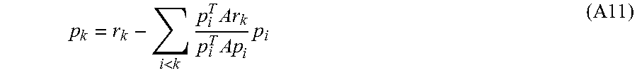
.function..times..times..times..di-elect cons. ##EQU00006## and as this function f becomes smaller, solution x gets closer to x*. The search (descent) direction for function f in (A9) equals to the negative gradient b-Ax. Starting from a guessed solution x.sub.0 (x.sub.0=0 in case of no guessed solution) at the k.sup.th step, this descent direction is r.sub.k=b-Ax.sub.k (A10) The conjugation constraint described previously is an orthonormal-type constraint and hence the algorithm bears resemblance to Gram-Schmidt orthonormalization. This gives the following expression for conjugate of r.sub.k
<.times..times..times..times. ##EQU00007## Following this direction, the next optimal location is
.alpha..times..times..times..alpha..times..times..times..times..times..ti- mes. ##EQU00008## where the last equality holds because p.sub.k and x.sub.k-1 are conjugate.
Conjugate Gradient Algorithm
The above algorithm gives the straightforward explanation of the conjugate gradient method. Seemingly, the algorithm as stated requires storage of all previous searching directions and residue vectors, as well as many matrix-vector multiplications, and thus can be computationally expensive. However, a closer analysis of the algorithm shows that r.sub.k+1 is conjugate to p.sub.i for all i<k, and therefore only r.sub.k, p.sub.k, and x.sub.k are needed to construct r.sub.k+1, p.sub.k+1, and x.sub.k+1. Furthermore, only one matrix-vector multiplication is needed in each iteration.
A modified algorithm is detailed below for solving Ax=b where A is a real, symmetric, positive-definite matrix, with an input vector x.sub.0 (a guessed solution otherwise 0).
TABLE-US-00002 Algorithm A1: A conjugate gradient algorithm. r.sub.0 = b - Ax.sub.0 p.sub.0 = r.sub.0 k = 0 REPEAT .alpha..times..times. ##EQU00009## x.sub.k+1 = x.sub.k + .alpha..sub.kp.sub.k r.sub.k+1 = r.sub.k - .alpha..sub.kAp.sub.k IF r.sub.k+1 is sufficiently small, EXIT REPEAT .beta..times..times. ##EQU00010## p.sub.k+1 = r.sub.k+1 + .beta..sub.kp.sub.k k = k + 1 END REPEAT RETURN x.sub.k+1
Preconditioned Conjugate Gradient Method
Preconditioning speeds up convergence of the conjugate gradient method. A preconditioned conjugate gradient algorithm is given in Algorithm A2, which requires an application of preconditioner operator B.sup.-1 on a given vector in addition to the steps in Algorithm A1.
TABLE-US-00003 Algorithm A2: A preconditioned conjugate gradient algorithm. r.sub.0 = b - Ax.sub.0 z.sub.0 = B.sup.-1r.sub.0 p.sub.0 = z.sub.0 k = 0 REPEAT .alpha..times..times. ##EQU00011## x.sub.k+1 = x.sub.k + .alpha..sub.kp.sub.k r.sub.k+1 = r.sub.k - .alpha..sub.kAp.sub.k IF r.sub.k+1 is sufficiently small, EXIT REPEAT z.sub.k+1 = B.sup.-1r.sub.k+1 .beta..times..times. ##EQU00012## p.sub.k+1 = r.sub.k+1 + .beta..sub.kp.sub.k k = k +1 END REPEAT RETURN x.sub.k+1
The preconditioner matrix B has to be symmetric positive-definite and fixed, i.e., cannot change from iteration to iteration. If any of these assumptions on the preconditioner is violated, the behavior of Algorithm A2 becomes unpredictable and its convergence can not be guaranteed.
Flexible Preconditioned Conjugate Gradient Method
For some numerically challenging applications, Algorithm A2 can be modified to accept variable preconditioners, changing between iterations, in order to improve the convergence performance of Algorithm A2. For instance, the Polak-Ribiere formula
.beta..function..times. ##EQU00013## instead of the Fletcher-Reeves formula used in Algorithm A2,
.beta..times..times. ##EQU00014## may dramatically improve the convergence of the preconditioned conjugate-gradient method. This version of the preconditioned conjugate gradient method can be called flexible, as it allows for variable preconditioning. The implementation of the flexible version requires storing an extra vector. For a fixed preconditioner, z.sub.k+1.sup.Tt.sub.k=0 both Polak-Ribiere and Fletcher-Reeves formulas are equivalent. The mathematical explanation of the better convergence behavior of the method with the Polak-Ribiere formula is that the method is locally optimal in this case, in particular, it does not converge slower than the locally optimal steepest descent method.
* * * * *
D00000
D00001
D00002
M00001
M00002
M00003
M00004
M00005
M00006
M00007
M00008
M00009
M00010

M00011

M00012
M00013

M00014

P00001

P00002

P00003

P00004

XML
uspto.report is an independent third-party trademark research tool that is not affiliated, endorsed, or sponsored by the United States Patent and Trademark Office (USPTO) or any other governmental organization. The information provided by uspto.report is based on publicly available data at the time of writing and is intended for informational purposes only.
While we strive to provide accurate and up-to-date information, we do not guarantee the accuracy, completeness, reliability, or suitability of the information displayed on this site. The use of this site is at your own risk. Any reliance you place on such information is therefore strictly at your own risk.
All official trademark data, including owner information, should be verified by visiting the official USPTO website at www.uspto.gov. This site is not intended to replace professional legal advice and should not be used as a substitute for consulting with a legal professional who is knowledgeable about trademark law.