FWI model domain angle stacks with amplitude preservation
Yang , et al. Dec
U.S. patent number 10,520,619 [Application Number 15/251,298] was granted by the patent office on 2019-12-31 for fwi model domain angle stacks with amplitude preservation. This patent grant is currently assigned to ExxonMobil Upstream Research Company. The grantee listed for this patent is Reeshidev Bansal, Anatoly I. Baumstein, Spyridon K. Lazaratos, Jia Yan, Di Yang. Invention is credited to Reeshidev Bansal, Anatoly I. Baumstein, Spyridon K. Lazaratos, Jia Yan, Di Yang.


| United States Patent | 10,520,619 |
| Yang , et al. | December 31, 2019 |
FWI model domain angle stacks with amplitude preservation
Abstract
A method, including: obtaining a seismic dataset that is separated into subsets according to predetermined subsurface reflection angle ranges; performing, with a computer, an acoustic full wavefield inversion process on each of the subsets, respectively, to invert for density and generate respective density models; generating acoustic impedances for each of the subsets, as a function of reflection angle, using the respective density models; and transforming, using a computer, the acoustic impedances for each of the subsets into reflectivity sections, wherein the transforming includes normalizing the reflectivity sections by their respective bandwidth.
| Inventors: | Yang; Di (Spring, TX), Bansal; Reeshidev (Spring, TX), Lazaratos; Spyridon K. (Houston, TX), Yan; Jia (Houston, TX), Baumstein; Anatoly I. (Houston, TX) | ||||||||||
|---|---|---|---|---|---|---|---|---|---|---|---|
| Applicant: |
|
||||||||||
| Assignee: | ExxonMobil Upstream Research
Company (Spring, TX) |
||||||||||
| Family ID: | 56889232 | ||||||||||
| Appl. No.: | 15/251,298 | ||||||||||
| Filed: | August 30, 2016 |
Prior Publication Data
| Document Identifier | Publication Date | |
|---|---|---|
| US 20170108602 A1 | Apr 20, 2017 | |
Related U.S. Patent Documents
| Application Number | Filing Date | Patent Number | Issue Date | ||
|---|---|---|---|---|---|
| 62241780 | Oct 15, 2015 | ||||
| Current U.S. Class: | 1/1 |
| Current CPC Class: | G01V 1/362 (20130101); G01V 1/282 (20130101); G01V 1/325 (20130101); E21B 41/0092 (20130101); G01V 2210/632 (20130101); G01V 2210/57 (20130101) |
| Current International Class: | G01V 1/28 (20060101); G01V 1/32 (20060101); G01V 1/36 (20060101); E21B 41/00 (20060101) |
References Cited [Referenced By]
U.S. Patent Documents
| 3812457 | May 1974 | Weller |
| 3864667 | February 1975 | Bahjat |
| 4159463 | June 1979 | Silverman |
| 4168485 | September 1979 | Payton et al. |
| 4545039 | October 1985 | Savit |
| 4562650 | January 1986 | Nagasawa et al. |
| 4575830 | March 1986 | Ingram et al. |
| 4594662 | June 1986 | Devaney |
| 4636957 | January 1987 | Vannier et al. |
| 4675851 | June 1987 | Savit et al. |
| 4686654 | August 1987 | Savit |
| 4707812 | November 1987 | Martinez |
| 4715020 | December 1987 | Landrum, Jr. |
| 4766574 | August 1988 | Whitmore et al. |
| 4780856 | October 1988 | Becquey |
| 4823326 | April 1989 | Ward |
| 4924390 | May 1990 | Parsons et al. |
| 4953657 | September 1990 | Edington |
| 4969129 | November 1990 | Currie |
| 4982374 | January 1991 | Edington et al. |
| 5260911 | November 1993 | Mason et al. |
| 5469062 | November 1995 | Meyer, Jr. |
| 5583825 | December 1996 | Carrazzone et al. |
| 5677893 | October 1997 | de Hoop et al. |
| 5715213 | February 1998 | Allen |
| 5717655 | February 1998 | Beasley |
| 5719821 | February 1998 | Sallas et al. |
| 5721710 | February 1998 | Sallas et al. |
| 5790473 | August 1998 | Allen |
| 5798982 | August 1998 | He et al. |
| 5822269 | October 1998 | Allen |
| 5838634 | November 1998 | Jones et al. |
| 5852588 | December 1998 | de Hoop et al. |
| 5878372 | March 1999 | Tabarovsky et al. |
| 5920838 | July 1999 | Norris et al. |
| 5924049 | July 1999 | Beasley et al. |
| 5999488 | December 1999 | Smith |
| 5999489 | December 1999 | Lazaratos |
| 6014342 | January 2000 | Lazaratos |
| 6021094 | February 2000 | Ober et al. |
| 6028818 | February 2000 | Jeffryes |
| 6058073 | May 2000 | VerWest |
| 6125330 | September 2000 | Robertson et al. |
| 6219621 | April 2001 | Hornbostel |
| 6225803 | May 2001 | Chen |
| 6311133 | October 2001 | Lailly et al. |
| 6317695 | November 2001 | Zhou et al. |
| 6327537 | December 2001 | Ikelle |
| 6374201 | April 2002 | Grizon et al. |
| 6381543 | April 2002 | Guerillot et al. |
| 6388947 | May 2002 | Washbourne et al. |
| 6480790 | November 2002 | Calvert et al. |
| 6522973 | February 2003 | Tonellot et al. |
| 6545944 | April 2003 | de Kok |
| 6549854 | April 2003 | Malinverno et al. |
| 6574564 | June 2003 | Lailly et al. |
| 6593746 | July 2003 | Stolarczyk |
| 6662147 | December 2003 | Fournier et al. |
| 6665615 | December 2003 | Van Riel et al. |
| 6687619 | February 2004 | Moerig et al. |
| 6687659 | February 2004 | Shen |
| 6704245 | March 2004 | Becquey |
| 6714867 | March 2004 | Meunier |
| 6735527 | May 2004 | Levin |
| 6754590 | June 2004 | Moldoveanu |
| 6766256 | July 2004 | Jeffryes |
| 6826486 | November 2004 | Malinverno |
| 6836448 | December 2004 | Robertsson et al. |
| 6842701 | January 2005 | Moerig et al. |
| 6859734 | February 2005 | Bednar |
| 6865487 | March 2005 | Charron |
| 6865488 | March 2005 | Moerig et al. |
| 6876928 | April 2005 | Van Riel et al. |
| 6882938 | April 2005 | Vaage et al. |
| 6882958 | April 2005 | Schmidt et al. |
| 6901333 | May 2005 | Van Riel et al. |
| 6903999 | June 2005 | Curtis et al. |
| 6905916 | June 2005 | Bartsch et al. |
| 6906981 | June 2005 | Vauge |
| 6927698 | August 2005 | Stolarczyk |
| 6944546 | September 2005 | Xiao et al. |
| 6947843 | September 2005 | Fisher et al. |
| 6970397 | November 2005 | Castagna et al. |
| 6977866 | December 2005 | Huffman et al. |
| 6999880 | February 2006 | Lee |
| 7046581 | May 2006 | Calvert |
| 7050356 | May 2006 | Jeffryes |
| 7069149 | June 2006 | Goff et al. |
| 7027927 | July 2006 | Routh et al. |
| 7072767 | July 2006 | Routh et al. |
| 7092823 | August 2006 | Lailly et al. |
| 7110900 | September 2006 | Adler et al. |
| 7184367 | February 2007 | Yin |
| 7230879 | June 2007 | Herkenoff et al. |
| 7271747 | September 2007 | Baraniuk et al. |
| 7330799 | February 2008 | Lefebvre et al. |
| 7337069 | February 2008 | Masson et al. |
| 7373251 | May 2008 | Hamman et al. |
| 7373252 | May 2008 | Sherrill et al. |
| 7376046 | May 2008 | Jeffryes |
| 7376539 | May 2008 | Lecomte |
| 7400978 | July 2008 | Langlais et al. |
| 7436734 | October 2008 | Krohn |
| 7480206 | January 2009 | Hill |
| 7525873 | April 2009 | Bush |
| 7584056 | September 2009 | Koren |
| 7599798 | October 2009 | Beasley et al. |
| 7602670 | October 2009 | Jeffryes |
| 7616523 | November 2009 | Tabti et al. |
| 7620534 | November 2009 | Pita et al. |
| 7620536 | November 2009 | Chow |
| 7646924 | January 2010 | Donoho |
| 7672194 | March 2010 | Jeffryes |
| 7672824 | March 2010 | Dutta et al. |
| 7675815 | March 2010 | Saenger et al. |
| 7679990 | March 2010 | Herkenhoff et al. |
| 7684281 | March 2010 | Vaage et al. |
| 7710821 | May 2010 | Robertsson et al. |
| 7715985 | May 2010 | Van Manen et al. |
| 7715986 | May 2010 | Nemeth et al. |
| 7725266 | May 2010 | Sirgue et al. |
| 7791980 | September 2010 | Robertsson et al. |
| 7835072 | November 2010 | Izumi |
| 7840625 | November 2010 | Candes et al. |
| 7940601 | May 2011 | Ghosh |
| 8121823 | February 2012 | Krebs et al. |
| 8248886 | August 2012 | Neelamani et al. |
| 8428925 | April 2013 | Krebs et al. |
| 8437998 | May 2013 | Routh et al. |
| 8547794 | October 2013 | Gulati et al. |
| 8688381 | April 2014 | Routh et al. |
| 8781748 | July 2014 | Laddoch et al. |
| 14329431 | July 2014 | Krohn et al. |
| 14330767 | July 2014 | Tang et al. |
| 8892413 | November 2014 | Routh |
| 2002/0049540 | April 2002 | Beve et al. |
| 2002/0099504 | July 2002 | Cross et al. |
| 2002/0120429 | August 2002 | Ortoleva |
| 2002/0183980 | December 2002 | Guillaume |
| 2004/0199330 | October 2004 | Routh et al. |
| 2004/0225438 | November 2004 | Okoniewski et al. |
| 2006/0104158 | May 2006 | Walls |
| 2006/0235666 | October 2006 | Assa et al. |
| 2007/0036030 | February 2007 | Baumel et al. |
| 2007/0038691 | February 2007 | Candes et al. |
| 2007/0274155 | November 2007 | Ikelle |
| 2008/0175101 | July 2008 | Saenger et al. |
| 2008/0306692 | December 2008 | Singer et al. |
| 2009/0006054 | January 2009 | Song |
| 2009/0067041 | March 2009 | Krauklis et al. |
| 2009/0070042 | March 2009 | Birchwood et al. |
| 2009/0083006 | March 2009 | Mackie |
| 2009/0164186 | June 2009 | Haase et al. |
| 2009/0164756 | June 2009 | Dokken et al. |
| 2009/0187391 | July 2009 | Wendt et al. |
| 2009/0248308 | October 2009 | Luling |
| 2009/0254320 | October 2009 | Lovatini et al. |
| 2009/0259406 | October 2009 | Khadhraoui et al. |
| 2010/0008184 | January 2010 | Hegna et al. |
| 2010/0018718 | January 2010 | Krebs et al. |
| 2010/0039894 | February 2010 | Abma et al. |
| 2010/0054082 | March 2010 | McGarry et al. |
| 2010/0088035 | April 2010 | Etgen et al. |
| 2010/0103772 | April 2010 | Eick et al. |
| 2010/0118651 | May 2010 | Liu et al. |
| 2010/0142316 | June 2010 | Keers et al. |
| 2010/0161233 | June 2010 | Saenger et al. |
| 2010/0161234 | June 2010 | Saenger et al. |
| 2010/0185422 | July 2010 | Hoversten |
| 2010/0208554 | August 2010 | Chiu et al. |
| 2010/0212902 | August 2010 | Baumstein et al. |
| 2010/0246324 | September 2010 | Dragoset, Jr. et al. |
| 2010/0265797 | October 2010 | Robertsson et al. |
| 2010/0270026 | October 2010 | Lazaratos et al. |
| 2010/0286919 | November 2010 | Lee et al. |
| 2010/0299070 | November 2010 | Abma |
| 2011/0000678 | January 2011 | Krebs et al. |
| 2011/0040926 | February 2011 | Donderici et al. |
| 2011/0051553 | March 2011 | Scott et al. |
| 2011/0075516 | March 2011 | Xia et al. |
| 2011/0090760 | April 2011 | Rickett et al. |
| 2011/0131020 | June 2011 | Meng |
| 2011/0134722 | June 2011 | Virgilio et al. |
| 2011/0182141 | July 2011 | Zhamikov et al. |
| 2011/0182144 | July 2011 | Gray |
| 2011/0191032 | August 2011 | Moore |
| 2011/0194379 | August 2011 | Lee et al. |
| 2011/0222370 | September 2011 | Downton et al. |
| 2011/0227577 | September 2011 | Zhang et al. |
| 2011/0235464 | September 2011 | Brittan et al. |
| 2011/0238390 | September 2011 | Krebs et al. |
| 2011/0246140 | October 2011 | Abubakar et al. |
| 2011/0267921 | November 2011 | Mortel et al. |
| 2011/0267923 | November 2011 | Shin |
| 2011/0276320 | November 2011 | Krebs et al. |
| 2011/0288831 | November 2011 | Tan et al. |
| 2011/0299361 | December 2011 | Shin |
| 2011/0320180 | December 2011 | Al-Saleh |
| 2012/0010862 | January 2012 | Costen |
| 2012/0014215 | January 2012 | Saenger et al. |
| 2012/0014216 | January 2012 | Saenger et al. |
| 2012/0051176 | March 2012 | Liu |
| 2012/0051177 | March 2012 | Hardage |
| 2012/0073824 | March 2012 | Routh |
| 2012/0073825 | March 2012 | Routh |
| 2012/0082344 | April 2012 | Donoho |
| 2012/0143506 | June 2012 | Routh et al. |
| 2012/0215506 | August 2012 | Rickett et al. |
| 2012/0218859 | August 2012 | Soubaras |
| 2012/0275264 | November 2012 | Kostov et al. |
| 2012/0275267 | November 2012 | Neelamani et al. |
| 2012/0290214 | November 2012 | Huo et al. |
| 2012/0314538 | December 2012 | Washbourne et al. |
| 2012/0316790 | December 2012 | Washbourne et al. |
| 2012/0316844 | December 2012 | Shah et al. |
| 2013/0028052 | January 2013 | Routh |
| 2013/0060539 | March 2013 | Baumstein |
| 2013/0081752 | April 2013 | Kurimura et al. |
| 2013/0238246 | September 2013 | Krebs et al. |
| 2013/0279290 | October 2013 | Poole |
| 2013/0282292 | October 2013 | Wang et al. |
| 2013/0311149 | November 2013 | Tang |
| 2013/0311151 | November 2013 | Plessix |
| 2014/0350861 | November 2014 | Wang et al. |
| 2014/0358504 | December 2014 | Baumstein et al. |
| 2014/0372043 | December 2014 | Hu et al. |
| 2016/0341858 | November 2016 | Magnusson |
| 2 796 631 | Nov 2011 | CA | |||
| 1 094 338 | Apr 2001 | EP | |||
| 1 746 443 | Jan 2007 | EP | |||
| 2 390 712 | Jan 2004 | GB | |||
| 2 391 665 | Feb 2004 | GB | |||
| WO 2006/037815 | Apr 2006 | WO | |||
| WO 2007/046711 | Apr 2007 | WO | |||
| WO 2008/042081 | Apr 2008 | WO | |||
| WO 2008/123920 | Oct 2008 | WO | |||
| WO 2009/067041 | May 2009 | WO | |||
| WO 2009/117174 | Sep 2009 | WO | |||
| WO 2010/085822 | Jul 2010 | WO | |||
| WO 2011/040926 | Apr 2011 | WO | |||
| WO 2011/091216 | Jul 2011 | WO | |||
| WO 2011/093945 | Aug 2011 | WO | |||
| WO 2012/024025 | Feb 2012 | WO | |||
| WO 2012/041834 | Apr 2012 | WO | |||
| WO 2012/083234 | Jun 2012 | WO | |||
| WO 2012/134621 | Oct 2012 | WO | |||
| WO 2012/170201 | Dec 2012 | WO | |||
| WO 2013/081752 | Jun 2013 | WO | |||
| WO-2015145257 | Oct 2015 | WO | |||
Other References
|
Frazer Barclay, Et Al, "Seismic Inversion: Reading Between the Lines", pp. 42-63, Oilfield Review (Year: 2008). cited by examiner . Aki, K and Richards, P (1980) Quantitative seismology, 2nd edition, University Science Books, pp. 133-155. cited by applicant . Dickens, T. A. et al. (2011) "RTM angle gathers using Poynting vectors", SEG Technical Program Expanded Abstracts 2011: pp. 3109-3113. cited by applicant . Sheriff, R.E. et al. (2002) Encyclopedic Dictionary of Applied Geophysics, 4th edition., SEG, pp. i-xii, 1-29. cited by applicant . Sheriff, R.E. et al. (2002) Encyclopedic Dictionary of Applied Geophysics, 4th edition., SEG, pp. i-xii, 400-402. cited by applicant . Xu, S., et al. (2011), "3D angle gathers from reverse time migration", Geophysics, vol. 76, No. 2, S77-S92. doi:10.1190/1.3536527. cited by applicant . Zhang, Y. et al. (2013) "A stable and practical implementation of least-squares reverse time migration". SEG Technical Program Expanded Abstracts 2013: pp. 3716-3720. cited by applicant . Mora, P. (1988) "Elastic wave-field inversion of reflection and transmission data" Geophysics, vol. 53, No. 6, pp. 750-759. cited by applicant . Morgan, J. et al. (2013) "Next-generation seismic experiments: wide-angle, multi-azimuth, three-dimensional, full-waveform inversion", Geophysical Journal International, Issue 195, pp. 1657-1678. cited by applicant . Shen, F. et al. (2002) "Effects of fractures on NMO velocities and P-wave azimuthal AVO response", Geophysics, vol. 67, No. 3, pp. 711-726. cited by applicant . Tang, B. et al. (2013) "3D angle gathers with plane-wave reverse-time migration", Geophysics, vol. 78, No. 2, pp. S117-S123. cited by applicant. |
Primary Examiner: Dalbo; Michael J
Attorney, Agent or Firm: ExxonMobil Upstream Research Company--Law Department
Parent Case Text
CROSS-REFERENCE TO RELATED APPLICATION
This application claims the benefit of U.S. Provisional Patent Application 62/241,780 filed Oct. 15, 2015 entitled FWI MODEL DOMAIN ANGLE STACKS WITH AMPLITUDE PRESERVATION, the entirety of which is incorporated by reference herein.
Claims
What is claimed is:
1. A method, comprising: obtaining a seismic dataset that is separated into subsets according to predetermined subsurface reflection angle ranges; performing, with a computer, an acoustic full wavefield inversion process on each of the subsets, respectively, to invert for density and generate respective density models; generating acoustic impedances for each of the subsets, as a function of reflection angle, using the respective density models; transforming, using a computer, the acoustic impedances for each of the subsets into reflectivity sections, wherein the transforming includes normalizing the reflectivity sections by their respective bandwidth; and using, for each of the reflectivity sections, a Fourier transform, discrete Fourier transform, or a fast Fourier transform to calculate an average spectrum within at least one local window that is applied at a same location to all of the reflectivity sections, and determining a bandwidth for each average spectrum.
2. The method of claim 1, wherein each of the full wavefield inversion processes start from a same velocity model.
3. The method of claim 1, wherein each of full wavefield inversion processes are independently applied to the subsets.
4. The method of claim 1, wherein the obtaining includes dividing a shot gather into the subsets by using a data mask that includes information of reflector dipping angles and P-wave velocity.
5. The method of claim 1, wherein the determining the bandwidth is based on a distance between 10-dB points.
6. The method of claim 1, wherein the determining the bandwidth is based on a distance between points with steepest slope.
7. The method of claim 1, wherein the average spectrum is calculated within a plurality of local windows, and is averaged.
8. The method of claim 1, further comprising determining reflectivity values at a plurality of angles and constructing an angle-vs-amplitude curve by interpolation.
9. The method of claim 1, further comprising managing hydrocarbon production using the reflectivity sections.
10. The method of claim 1, wherein the managing hydrocarbon production includes drilling a well at a location determined at least in part by the reflectivity sections.
11. A non-transitory computer readable storage medium encoded with instructions, which when executed by a computer cause the computer to implement a method comprising: obtaining a seismic dataset that is separated into subsets according to predetermined subsurface reflection angle ranges; performing, with a computer, an acoustic full wavefield inversion process on each of the subsets, respectively, to invert for density and generate respective density models; generating acoustic impedances for each of the subsets, as a function of reflection angle, using the respective density models; transforming, using a computer, the acoustic impedances for each of the subsets into reflectivity sections, wherein the transforming includes normalizing the reflectivity sections by their respective bandwidth; and using, for each of the reflectivity sections, a Fourier transform, discrete Fourier transform, or a fast Fourier transform to calculate an average spectrum within at least one local window that is applied at a same location to all of the reflectivity sections, and determining a bandwidth for each average spectrum.
Description
FIELD OF THE INVENTION
Exemplary embodiments described herein pertain to the field of geophysical prospecting, and more particularly to geophysical data processing. Specifically, embodiments described herein relate to a method for more efficiently generating FWI model domain angle stacks.
BACKGROUND
This section is intended to introduce various aspects of the art, which may be associated with exemplary embodiments of the present invention. This discussion is believed to assist in providing a framework to facilitate a better understanding of particular aspects of the present invention. Accordingly, it should be understood that this section should be read in this light, and not necessarily as admissions of prior art.
An important goal of seismic prospecting is to accurately image subsurface structures commonly referred to as reflectors. Seismic prospecting is facilitated by obtaining raw seismic data during performance of a seismic survey. During a seismic survey, seismic energy is generated at ground level by, for example, a controlled explosion, and delivered to the earth. Seismic waves are reflected from underground structures and are received by a number of sensors referred to as geophones. The seismic data received by the geophones is processed in an effort to create an accurate mapping of the underground environment. The processed data is then examined with a goal of identifying geological formations that may contain hydrocarbons.
Full Wavefield Inversion (FWI) is a geophysical method which is used to estimate subsurface properties (such as velocity or density). It is known to be advanced for the higher resolution and more accurate physics compared to conventional methods. The fundamental components of an FWI algorithm can be described as follows: using a starting subsurface physical properties model, synthetic seismic data are generated by solving a wave equation using a numerical scheme (e.g., finite-difference, finite-element etc.). The synthetic seismic data are compared with the field seismic data and using the difference between the two, the value of an objective function is calculated. To minimize the objective function, a modified subsurface model is generated which is used to simulate a new set of synthetic seismic data. This new set of synthetic seismic data is compared with the field data to recalculate the value of the objective function. The objective function optimization procedure is iterated by using the new updated model as the starting model for finding another search direction, which will then be used to perturb the model in order to better explain the observed data. The process continues until an updated model is found that satisfactorily explains the observed data. A global or local optimization method can be used to minimize the objective function and to update the subsurface model. Commonly used local objective function optimization methods include, but are not limited to, gradient search, conjugate gradients, quasi-Newton, Gauss-Newton and Newton's method. Commonly used global methods included, but are not limited to, Monte Carlo or grid search.
Although FWI is expected to provide the subsurface properties, it is difficult to extract the correct viscoelastic properties from the seismic data directly with FWI. As FWI estimates the properties by fitting the data with synthetic waveforms, it relies on how accurate the wave equation can explain the actual physics, and how well the optimization method can separate the effects from different properties. When an acoustic wave equation is used, FWI can generate P-wave velocity models based on the travel time information in the datasets. However, the amplitude information is not fully utilized because the real earth is visco-elastic, and an acoustic model cannot explain all the amplitudes in the acquired data. If FWI is expected to provide interpretable products like elastic impedances, elastic simulation is often needed but very expensive; in general it is 6 to 10 times the computation of acoustic FWI. In addition, the initial model for shear wave velocity is difficult to obtain due to the limited shear wave kinematic information and often poor signal to noise ratio in the acquisitions.
An alternative way of using the elastic amplitude information is to form angle stacks. Amplitude versus angle (AVA) analysis [5] can be performed on the angle stacks to extract the elastic properties. Traditional AVA stacks generated with Kirchhoff migration need geometric spreading corrections to account for the amplitude loss during propagation. However, it is not guaranteed that the amplitude after correction would reflect the true amplitude of the data. In addition, Kirchhoff migration is based on ray-tracing which favors smooth velocity models and would likely fail in high contrast medium. Angle calculations are under a 1-D assumption that is not accurate enough when subsurface structures are complex. Reverse time migration (RTM) based angle stacks [1, 2] are more advanced for making use of the high-resolution velocity models. Nonetheless, amplitude preservation is still difficult. Yu Zhang et al (2014) [3] reported a least-squares RTM to balance the image amplitudes; however, it has not been proved to be able to generate angle stacks.
SUMMARY
A method, including: obtaining a seismic dataset that is separated into subsets according to predetermined subsurface reflection angle ranges; performing, with a computer, an acoustic full wavefield inversion process on each of the subsets, respectively, to invert for density and generate respective density models; generating acoustic impedances for each of the subsets, as a function of reflection angle, using the respective density models; and transforming, using a computer, the acoustic impedances for each of the subsets into reflectivity sections, wherein the transforming includes normalizing the reflectivity sections by their respective bandwidth.
In the method, each of the full wavefield inversion processes start from a same velocity model.
In the method, each of full wavefield inversion processes are independently applied to the subsets.
In the method, the obtaining includes dividing a shot gather into the subsets by using a data mask that includes information of reflector dipping angles and P-wave velocity.
The method can further include using, for each of the reflectivity sections, a Fourier transform, discrete Fourier transform, or a fast Fourier transform to calculate an average spectrum within at least one local window that is applied at a same location to all of the reflectivity sections, and determining a bandwidth for each average spectrum.
In the method, the determining the bandwidth is based on a distance between 10-dB points.
In the method, the determining the bandwidth is based on a distance between points with steepest slope.
In the method, the average spectrum is calculated within a plurality of local windows, and is averaged.
The method can further include determining reflectivity values at a plurality of angles and constructing an angle-vs-amplitude curve by interpolation.
The method can further include managing hydrocarbon production using the reflectivity sections.
In the method, the managing hydrocarbon production includes drilling a well at a location determined at least in part by the reflectivity sections.
A non-transitory computer readable storage medium encoded with instructions, which when executed by a computer cause the computer to implement a method including: obtaining a seismic dataset that is separated into subsets according to predetermined subsurface reflection angle ranges; performing, with a computer, an acoustic full wavefield inversion process on each of the subsets, respectively, to invert for density and generate respective density models; generating acoustic impedances for each of the subsets, as a function of reflection angle, using the respective density models; and transforming, using a computer, the acoustic impedances for each of the subsets into reflectivity sections, wherein the transforming includes normalizing the reflectivity sections by their respective bandwidth.
BRIEF DESCRIPTION OF THE DRAWINGS
While the present disclosure is susceptible to various modifications and alternative forms, specific example embodiments thereof have been shown in the drawings and are herein described in detail. It should be understood, however, that the description herein of specific example embodiments is not intended to limit the disclosure to the particular forms disclosed herein, but on the contrary, this disclosure is to cover all modifications and equivalents as defined by the appended claims. It should also be understood that the drawings are not necessarily to scale, emphasis instead being placed upon clearly illustrating principles of exemplary embodiments of the present invention. Moreover, certain dimensions may be exaggerated to help visually convey such principles.
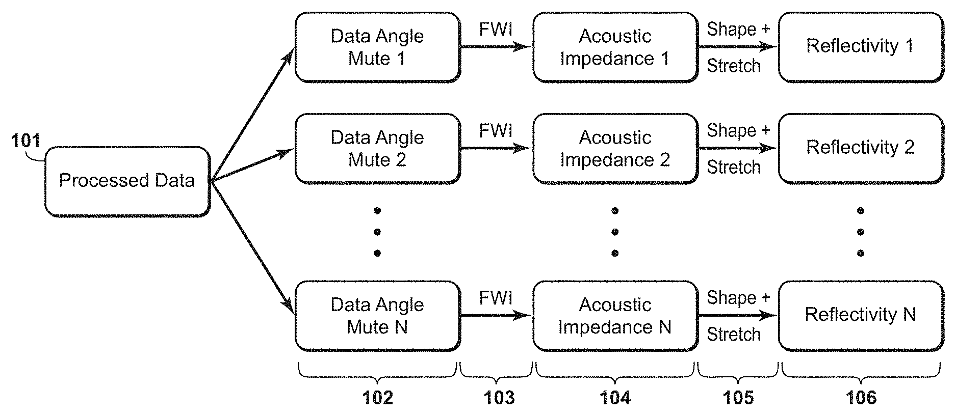
FIG. 1 illustrates an exemplary method for generating FWI AVA stacks.
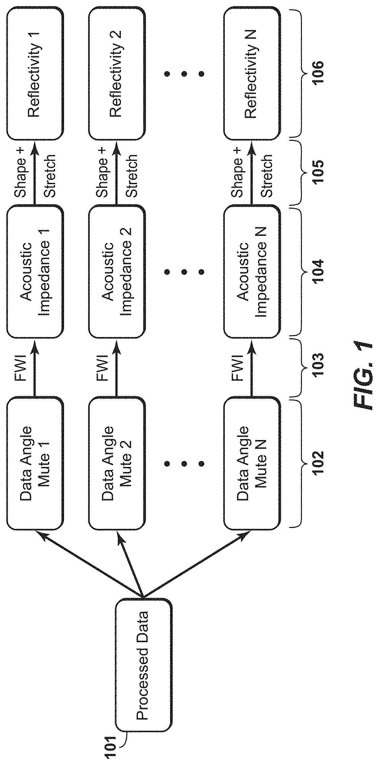
FIG. 2 illustrates the spectrum spreading effect due to scattering angles.
FIG. 3A illustrates a single shot gather.
FIG. 3B illustrates the single shot gather that is muted into five different angle ranges.
FIG. 4A illustrates angle stacks with acoustic FWI.
FIG. 4B illustrates angle stacks with convolutions.
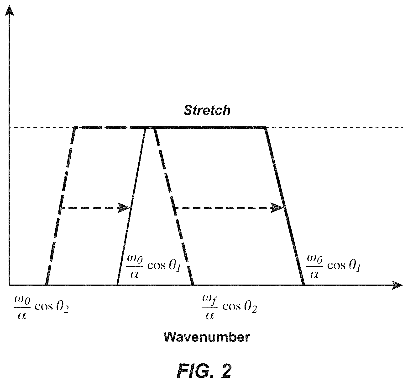
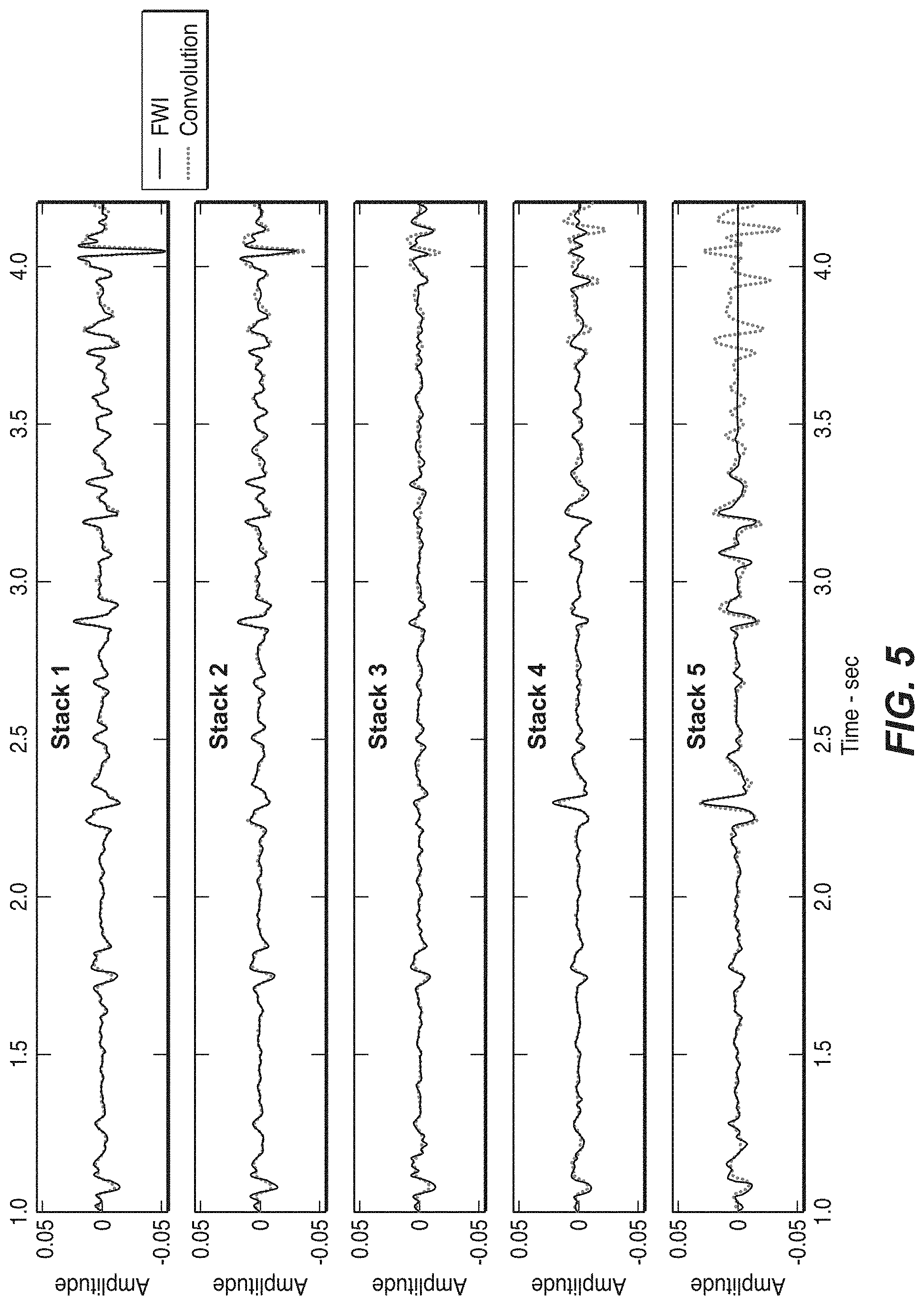
FIG. 5 illustrates the vertical lines from each angle stack in FIGS. 4A and 4B, overlaid to show consistency.
DETAILED DESCRIPTION
Exemplary embodiments are described herein. However, to the extent that the following description is specific to a particular embodiment, this is intended to be for exemplary purposes only and simply provides a description of the exemplary embodiments. Accordingly, the invention is not limited to the specific embodiments described below, but rather, it includes all alternatives, modifications, and equivalents falling within the true spirit and scope of the appended claims.
Exemplary embodiments described herein provide a method than can: 1) be robust with complex geology; 2) preserve the amplitude versus angle information; and 3) be less expensive than elastic FWI. The proposed FWI model domain angle stacks can be generated by inverting the datasets of different angle ranges for different acoustic models. Amplitude preservation can be achieved through the data fitting process, and the angle calculation is more accurate using Poynting vectors. The Poynting vector describes energy flow for body waves, interface waves, guided waves and inhomogeneous waves in isotropic and anisotropic media. Poynting vectors naturally take the advantage of the high-resolution FWI velocity models. When implemented as an integrated part of a FWI workflow, the present technological advantage can utilize the FWI products angle stacks without changing platforms. More importantly, exemplary method are not limited to the incomplete physics in the modeling engine.
Exemplary embodiments of the present technological advancement generates model domain amplitude preserved angle stacks using FWI. Advantageously, the present technological advancement can use only acoustic simulations, but can be applied to the full offsets of the acquired seismic data. It is impossible to use one acoustic model to fit all the data that contains all kinds of physics. However, if the datasets are separated by the reflection angles, for each angle, there is an acoustic model that can explain the data. With all the models combined, an impedance model is formed as a function of reflection angle: I(.theta.). Acoustic impedance is a measure of the ease with which seismic energy travels through a particular portion of the subsurface environment. Those of ordinary skill in the art will appreciate that acoustic impedance may be defined as a product of density and seismic velocity. From the impedance, the reflectivity can be derived as a function of angle: R(.theta.), which is exactly the definition of AVA.
In practice, it is not necessary to find a continuous form of R(.theta.). Instead, R(.theta.) can be determined at several angles, and the AVA curve can be reconstructed by interpolation.
FIG. 1 illustrates an exemplary method for generating FWI AVA stacks. In step 101, processed data is obtained, which can be a single shot gather generated from the collected seismic data. Such processed data is seismic data conditioned according to conventional techniques known to those of ordinary skill in the art. In step 102, the shot gather is divided into several subsets. Each subset is within a relatively small range of reflection angles. This can be achieved by using carefully designed data masks which include the information of reflector dipping angles and P-wave velocity. With the dipping angles and P-wave velocity, a ray-tracing method can be used to find the time and offset of the reflected wave in the data from each of the subsurface points at each reflection angle. Data masking is a process of hiding a portion of the original data so that only the desired portion (i.e., desired angle range) is available for subsequent processing. The angle ranges shown in the accompanying figures are only exemplary, and other angle ranges can be used. Moreover, the number of angle ranges is also exemplary as the shot gather could be divided in to more or less sections.
In step 103, on each of the data subsets generated in step 102, acoustic FWI is applied to obtain acoustic impedances independently. Those of ordinary skill in the art are familiar with acoustic FWI and further details of this process are omitted. All inversions can start from the same velocity model, and the kinematics are not updated in this process assuming that velocity model building is already finished and accurate enough. The model updates are meant to explain the data amplitude only. After the inversion, the synthetic waveforms simulated with these impedances fit the real data well so that the amplitude information is preserved in the model domain. Each impedance model can only explain the data of a certain range of reflection angles constrained by the data masks. Within one angle range, the mid angle can be chosen to be the nominal angle of the reflectivity. This is additionally guaranteed by using Poynting vectors [2] when forming the gradient in the inversion, and so the gradient is most sensitive to the reflections at the nominal angle. Poynting vectors are used to separate the wave propagation directions during the finite difference simulation and gradient calculation. The data separation can be conducted based on ray-theory. Since the Poynting vector is based on wave-theory, it can be a helpful check on the accuracy of the data separation.
The term velocity model, density model, or physical property model as used herein refers to an array of numbers, typically a 3-D array, where each number, which may be called a model parameter, is a value of velocity, density or another physical property in a cell, where a subsurface region has been conceptually divided into discrete cells for computational purposes.
After the inversion, both density and velocity are known and step 104 can determine impedance from the results of the acoustic FWI as impedance is a function of density and velocity.
In acoustic FWI, two parameters can be inverted for to fit the data amplitudes: P-wave velocity and density. P-wave velocity is often chosen to fit the amplitude and travel time at the same time when an L-2 norm type of objective function is used. However, density may be a better parameter for reflectivity inversion. Density has a much simpler AVA response than P-wave velocity. As described in the Aki-Richards equation:
.function..theta..times..DELTA..times..times..rho..rho..times..times..the- ta..times..DELTA..times..times..alpha..alpha. ##EQU00001## where .DELTA.p is density perturbation and Act is the P-wave velocity perturbation, density has a constant AVA response which does not vary with angle [6]. This indicates that when a density perturbation is inverted for to fit the data amplitude at a certain angle .theta., the value of the perturbation directly represents the reflectivity at that angle .theta. regardless of the actual value of .theta.. On the contrary, if a P-wave velocity perturbation is used, in order to obtain R(.theta.), we need to apply a correction of
.times..times..theta. ##EQU00002## Moreover, Equation [1] is only valid when the perturbation is weak, and when the perturbation is strong, the correction does not have an explicit form. For density, the constant AVA response is valid for all cases.
After the acoustic impedances are obtained, they can be shaped or converted into reflectivity sections (P-P reflectivity) in step 105. The reflectivity sections can be approximately determined from the derivative of the acoustic impedance with respect to space (or more generally the vertical derivative, which in some cases could be time). However, there is one more step to balance the reflectivity spectrum across different angles, i.e., "stretch". While FIG. 1 shows "shape" and "stretch" in the same step, these are not necessarily performed simultaneously.
Similar to the wavelet stretching effect in migration, the reflectivity's obtained from data of different reflection angles are of different resolutions. Because there is only bandlimited data (.omega..sub.0.about..omega..sub.f), where .omega..sub.0 and .omega..sub.f are the minimum and maximum frequencies present in the data, at each angle .theta. the reflectivity spectrum is only sampled from
.omega..alpha..times..times..times..theta..times..times..times..times..om- ega..alpha..times..times..times..theta. ##EQU00003## in the wavenumber domain as shown in FIG. 2. Different bandwidth in the wavenumber domain leads to different amplitude in the space domain. Assuming the true reflectivity values R(.theta..sub.1) and R(.theta..sub.2) are the same, the relation between the inverted reflectivities would be
.function..theta..function..theta..times..times..theta..times..times..the- ta. ##EQU00004## Therefore, to preserve the data AVO in the model domain, there is a need to compensate the spectrum stretch by dividing by a factor of cos .theta.. In practice, it is difficult to use data of a single reflection angle. Therefore, an alternative way of obtaining the compensation factor is to measure the bandwidth of the reflectivity. For all the reflectivity sections, a Fourier transform can be used to calculate the averaged spectrum within a local window that is applied at the same location to all sections. This can be performed at multiple locations and averaged, as long as the locations are the same in all sections. The Fourier transform may be preferred, but other transforms could be used, such as FFT or DFT. The bandwidth can be defined, for example, as the distance between the 10-dB points. However, other measures of bandwidth can be used (i.e., 3-dB points, full-width half maximum, points of steepest slope, etc.), but the distance between the 10-dB points may be preferred. Then, to complete step 105 and compensate for the "stretch," each reflectivity section is normalized by its own bandwidth so that the spectrum stretching effect on the reflectivity amplitude is corrected for.
The final output of the method in FIG. 1 (step 106) are the reflectivity stacks for different angles.
The present technological advancement was applied on a synthetic dataset generated with a 2-D slice extracted from the SEG SEAM Phase I model. Pressure data are simulated with streamers of 4 km maximum offset. An absorbing boundary condition is used on the water surface. Therefore, no free surface related multiples are present in the data. As shown in FIG. 3A, a single shot gather is divided into five sections by the dashed lines 301, 302, 303, 304, and 305, which corresponds to the following angle ranges: 0-10; 10-20; 20-30; 30-40; and 40-50 degrees. The angle ranges do not necessarily need to overlap. Five data masks are designed based on these lines 301-305, each covering 10 degrees of reflection angle. Therefore, five data subsets are generated (see step 102) as shown in FIG. 3B. Starting from the same velocity model, acoustic FWI was performed (see step 103) using each of the subsets respectively. The resulting acoustic impedances (see step 104) after the inversion are "shaped" and "stretched" (see step 105) into reflectivity sections (see step 106), and shown in the panels in FIG. 4A. The gap area 401 in the last panel is because the large angle reflection from the deep part is outside of the acquisition offset. To verify the quality of the results, true reflectivity sections are generated by the convolution between the seismic wavelet and the reflectivity sequences, and are shown in FIG. 4B. The reflectivity sequences are calculated using the Zoeppritz equation [4] and the true synthetic model. The AVA in FIGS. 4A and 4B appears to be consistent. For a closer scrutiny, five vertical lines 402a, 403a, 404a, 405a, and 406a from the model domain stacks, and five from the convolution sections 402b, 403b, 404b, 405b, and 406b are overlaid in FIG. 5 to show the consistency. It is clear that at all angles and all depths the FWI model domain stacks have very similar amplitudes compared to the convolution stacks. It demonstrates that the workflow is reliable and accurate with a complicated geology.
The final reflectivity's are an example of a subsurface image that can be used for interpretation of the subsurface and/or management of hydrocarbon exploration. As used herein, hydrocarbon management includes hydrocarbon extraction, hydrocarbon production, hydrocarbon exploration, identifying potential hydrocarbon resources, identifying well locations, determining well injection and/or extraction rates, identifying reservoir connectivity, acquiring, disposing of and/or abandoning hydrocarbon resources, reviewing prior hydrocarbon management decisions, and any other hydrocarbon-related acts or activities.
In all practical applications, the present technological advancement must be used in conjunction with a computer, programmed in accordance with the disclosures herein. Preferably, in order to efficiently perform FWI, the computer is a high performance computer (HPC), known as to those skilled in the art, Such high performance computers typically involve clusters of nodes, each node having multiple CPU's and computer memory that allow parallel computation. The models may be visualized and edited using any interactive visualization programs and associated hardware, such as monitors and projectors. The architecture of system may vary and may be composed of any number of suitable hardware structures capable of executing logical operations and displaying the output according to the present technological advancement. Those of ordinary skill in the art are aware of suitable supercomputers available from Cray or IBM.
REFERENCES
The following references are hereby incorporated by reference in their entirety:
[1] Xu, S., Y. Zhang and B. Tang, 2011, 3D angle gathers from reverse time migration: Geophysics, 76:2, S77-S92. doi:10.1190/1.3536527;
[2] Thomas A. Dickens and Graham A. Winbow (2011) RTM angle gathers using Poynting vectors. SEG Technical Program Expanded Abstracts 2011: pp. 3109-3113;
[3] Yu Zhang, Lian Duan, and Yi Xie (2013) A stable and practical implementation of least-squares reverse time migration. SEG Technical Program Expanded Abstracts 2013: pp. 3716-3720;
[4] Encyclopedic Dictionary of Applied Geophysics, R. E. Sheriff, 4.sup.th edition., SEG, 2002, p. 400;
[5] Encyclopedic Dictionary of Applied Geophysics, R. E. Sheriff, 4th edition., SEG, 2002, p. 12; and
[6] Aki, K and Richards, P (1980) Quantitative seismology, 2nd edition, University Science Books, p. 133-155.
* * * * *
D00000
D00001
D00002
D00003
D00004
M00001
M00002
M00003
M00004
XML
uspto.report is an independent third-party trademark research tool that is not affiliated, endorsed, or sponsored by the United States Patent and Trademark Office (USPTO) or any other governmental organization. The information provided by uspto.report is based on publicly available data at the time of writing and is intended for informational purposes only.
While we strive to provide accurate and up-to-date information, we do not guarantee the accuracy, completeness, reliability, or suitability of the information displayed on this site. The use of this site is at your own risk. Any reliance you place on such information is therefore strictly at your own risk.
All official trademark data, including owner information, should be verified by visiting the official USPTO website at www.uspto.gov. This site is not intended to replace professional legal advice and should not be used as a substitute for consulting with a legal professional who is knowledgeable about trademark law.