Analysis of failures in combinatorial test suite
Lekivetz , et al.
U.S. patent number 10,338,993 [Application Number 16/154,290] was granted by the patent office on 2019-07-02 for analysis of failures in combinatorial test suite. This patent grant is currently assigned to SAS Institute Inc.. The grantee listed for this patent is SAS Institute Inc.. Invention is credited to Bradley Allen Jones, Ryan Adam Lekivetz, Joseph Albert Morgan.


View All Diagrams
| United States Patent | 10,338,993 |
| Lekivetz , et al. | July 2, 2019 |
Analysis of failures in combinatorial test suite
Abstract
The computing device generates a test suite that provides test cases for testing a system. A test condition in the test suite comprises one of different levels representing different options assigned to a categorical factor for the system. The computing device receives input weights for one or more levels of the test suite. The computing device receives a failure indication indicating a test conducted according to the test cases failed. The computing device determines a plurality of cause indicators based on the input weights and any commonalities between test conditions of any failed test cases of the test suite that resulted in a respective failed test outcome. The computing device identifies, based on comparing the plurality of cause indicators, a most likely potential cause for a potential failure of the system. The computing device outputs an indication of the most likely potential cause for the potential failure of the system.
| Inventors: | Lekivetz; Ryan Adam (Cary, NC), Morgan; Joseph Albert (Raleigh, NC), Jones; Bradley Allen (Cary, NC) | ||||||||||
|---|---|---|---|---|---|---|---|---|---|---|---|
| Applicant: |
|
||||||||||
| Assignee: | SAS Institute Inc. (Cary,
NC) |
||||||||||
| Family ID: | 67069451 | ||||||||||
| Appl. No.: | 16/154,290 | ||||||||||
| Filed: | October 8, 2018 |
Related U.S. Patent Documents
| Application Number | Filing Date | Patent Number | Issue Date | ||
|---|---|---|---|---|---|
| 62702247 | Jul 23, 2018 | ||||
| 62661057 | Apr 22, 2018 | ||||
| Current U.S. Class: | 1/1 |
| Current CPC Class: | G06F 11/0709 (20130101); G06F 11/3684 (20130101); G06F 11/321 (20130101); G06N 20/00 (20190101); G06F 11/0739 (20130101); G06F 11/3692 (20130101); G06F 11/263 (20130101); G06N 3/0445 (20130101); G06F 11/3688 (20130101); G06F 11/261 (20130101); G06N 3/084 (20130101); G06F 11/0766 (20130101); G06N 3/063 (20130101); G06F 11/3664 (20130101); G06F 11/079 (20130101); G06F 11/3409 (20130101); G06F 11/2028 (20130101) |
| Current International Class: | G06F 11/00 (20060101); G06F 11/07 (20060101); G06F 11/26 (20060101); G06F 11/34 (20060101); G06F 11/36 (20060101) |
References Cited [Referenced By]
U.S. Patent Documents
| 8019049 | September 2011 | Allen, Jr. |
| 8495583 | July 2013 | Bassin |
| 8756460 | June 2014 | Blue |
| 9218271 | December 2015 | Segall |
| 9529700 | December 2016 | Raghavan |
| 2003/0233600 | December 2003 | Hartman |
| 2008/0256392 | October 2008 | Garland |
| 2015/0309918 | October 2015 | Raghavan |
| 2016/0299836 | October 2016 | Kuhn |
| 2017/0103013 | April 2017 | Grechanik |
Other References
|
Kuhn et al. "Software Fault Interactions and Implications for Software Testing"; IEEE Transaction on Software Engineering; Jun. 2004; pp. 418-421; vol. 30, No. 6. cited by applicant . Bryce et al. "Prioritized interaction testing for pair-wise coverage with seeding and constraints"; Information and Software Technology; Feb. 27, 2006; pp. 960-970; vol. 48, No. 10. cited by applicant . Chandrasekaran et al. "Evaluating the effectiveness of BEN in localizing different types of software fault"; IEEE 9th International Conference on Software Testing, Verification and Validation Workshops; Apr. 10, 2016; pp. 1-31. cited by applicant . Colbourn et al. "Locating and Detecting Arrays for Interaction Faults"; Journal of Combinatorial Optimization; 2008; pp. 1-34; vol. 15, No. 1. cited by applicant . Dalal et al. "Factor-Covering Designs for Testing Software"; Technometrics; Aug. 1998; pp. 1-14; vol. 40, No. 3. cited by applicant . Demiroz et al. "Cost-Aware Combinatorial Interaction Testing"; Proc. of the International Conference on Advanaces in System Testing and Validation Lifecycles; 2012; pp. 1-8. cited by applicant . Elbaum et al. "Selecting a Cost-Effective Test Case Prioritization Technique"; Software Quality Journal; Apr. 20, 2004; pp. 1-26; vol. 12, No. 3. cited by applicant . Ghandehari et al. "Identifying Failure-Inducing Combinations in a Combinatorial Test Set"; IEEE Fifth International Conference on Software Testing, Verification and Validation; Apr. 2012; pp. 1-10. cited by applicant . Ghandehari et al. "Fault Localization Based on Failure-Inducing Combinations"; IEEE 24th International Symposium on Software Reliability Engineering; Nov. 2013; pp. 168-177. cited by applicant . Alan Hartman "Software and Hardware Testing Using Combinatorial Covering Suites"; The Final Draft; Jul. 3, 2018; pp. 1-41; IBM Haifa Research Laboratory. cited by applicant . Katona et al. "Two Applications (for Search Theory and Truth Functions) of Spemer Type Theorems"; Periodica Mathematica Hungarica; 1973; pp. 19-26; vol. 3, No. 1-2. cited by applicant . Cohen et al. "Interaction Testing of Highly-Configurable Systems in the Presence of Constraints"; ISSTA '07 London, England, United Kingdom; Jul. 9-12, 2007; pp. 1-11; ACM 978-1-59593-734-6/07/0007. cited by applicant . Cohen et al. "The Combinatorial Design Approach to Automatic Test Generation"; IEEE Software; Sep. 1996; pp. 83-88; vol. 13, No. 5. cited by applicant . Dunietz et al. "Applying Design of Experiments to Software Testing"; Proceedings of 19th ECSE, New York, NY; 1997; pp. 205-215; ACM, Inc. cited by applicant . Cohen et al. "The AETG System: An Approach to Testing Based on Combinatorial Design"; IEEE Transactions on Software Engineering; Jul. 1997; pp. 437-444; vol. 23, No. 7. cited by applicant . Joseph Morgan "Combinatorial Testing: An Approach to Systems and Software Testing Based on Covering Arrays"; Book--Analytic Methods in Systems and Software Testing; 2018; pp. 131-158; John Wiley & Sons Ltd.; Hoboken, NJ, US. cited by applicant . Cohen et al. "Constructing Interaction Test Suites for Highly-Configurable Systems in the Presence of Constraints: A Greedy Approach"; IEEE Transactions on Software Engineering; Sep./Oct. 2008; pp. 633-650; vol. 34, No. 5. cited by applicant . Colbourn et al. "Coverage, Location, Detection, and Measurement"; IEEE Ninth International Conference on Software Testing, Verification and Validation Workshops; Apr. 2016; pp. 19-25. cited by applicant . Kleitman et al. "Families of .kappa.-Independent Sets"; Discrete Mathematics; 1973; pp. 255-262; vol. 6, No. 3. cited by applicant . Johnson et al. "Largest Induced Subgraphs of the n-Cube That Contain No 4-Cycles"; Journal of Combinatorial Theory; 1989; pp. 346-355; Series B 46. cited by applicant . Dalal et al. "Model-Based Testing in Practice"; Proceedings of the 21st ICSE, New York, NY; 1999; pp. 1-10. cited by applicant . Moura et al. "Covering Arrays with Mixed Alphabet Sizes"; Journal of Combinatorial Design; 2003; pp. 413-432; vol. 11, No. 6. cited by applicant . Brownlie et al. "Robust Testing of AT&T PMX/StarMAIL Using OATS"; AT&T Technical Journal, May 1992; pp. 41-47; vol. 73, No. 3. cited by applicant . Robert Mandl "Orthogonal Latin Squares: an Application of Experiment Design to Compiler Testing"; Communications of the ACM; Oct. 1985; pp. 1054-1058; vol. 28, No. 10. cited by applicant . Hartman et al. "Problems and algorithms for covering arrays"; Discrete Mathematics; 2004; pp. 149-156; vol. 284, No. 1-3. cited by applicant. |
Primary Examiner: Bonzo; Bryce P
Assistant Examiner: Gibson; Jonathan D
Attorney, Agent or Firm: Coats & Bennett, PLLC
Parent Case Text
RELATED APPLICATIONS
This application claims the benefit of U.S. Provisional Application No. 62/702,247 filed Jul. 23, 2018, and claims the benefit of U.S. Provisional Application No. 62/661,057, filed Apr. 22, 2018, the disclosures of which are incorporated herein by reference in their entirety.
Claims
What is claimed is:
1. A computer-program product tangibly embodied in a non-transitory machine-readable storage medium, the computer-program product including instructions operable to cause a computing device to: generate a test suite that provides test cases for testing a system comprising different components, wherein each element of a test case of the test suite is a test condition for testing one of categorical factors for the system, each of the categorical factors representing one of the different components, and wherein a test condition in the test suite comprises one of different levels representing different options assigned to a categorical factor for the system; receive a set of input weights for one or more levels of the test suite; receive a failure indication indicating a test conducted according to the test cases failed; in response to receiving the failure indication, determine a plurality of cause indicators based on the set of input weights and any commonalities between test conditions of any failed test cases of the test suite that resulted in a respective failed test outcome, wherein each cause indicator represents a likelihood that a test condition or combination of test conditions of the any failed test cases caused the respective failed test outcome; identify, based on comparing the plurality of cause indicators, a most likely potential cause for a potential failure of the system; and output an indication of the most likely potential cause for the potential failure of the system.
2. The computer-program product of claim 1, wherein the system comprises a software program, wherein the categorical factors comprise a component that models an operation of the software program, and wherein the instructions are operable to cause the computing device to test each of the test cases of the test suite by executing the software program on computer hardware using respective test conditions of the respective test case.
3. The computer-program product of claim 2, wherein the failure indication indicates that executing the software program using the respective test conditions did not operate in accordance with a set of predefined behaviors for the software program.
4. The computer-program product of claim 1, wherein the system is a deterministic computer-simulated model representing behavior of computer hardware.
5. The computer-program product of claim 1, wherein the system comprises computer hardware and a first categorical factor of the categorical factors represents a circuit of the system configured to implement aspects of the computer hardware.
6. The computer-program product of claim 1, wherein the instructions are operable to cause the computing device to: receive the set of input weights by displaying a first graphical user interface for user entry of the set of input weights; and output the indication to a display device to display a second graphical user interface for displaying the indication.
7. The computer-program product of claim 1, wherein the instructions are operable to cause the computing device to: receive one or more failure indications indicating a plurality of tests conducted according to the test cases failed; determine commonalities of test conditions between one or more of the plurality of tests that failed; and assign a value to a cause indicator of the plurality of cause indicators that accounts for one or more of the determined commonalities.
8. The computer-program product of claim 1, wherein the instructions are operable to cause the computing device to identify the most likely potential cause by generating an ordered ranking of the plurality of cause indicators for further testing of the system and output the indication by outputting the ordered ranking.
9. The computer-program product of claim 1, wherein the set of input weights are generated based on prior performance in testing the system or another system.
10. The computer-program product of claim 1, wherein the instructions are operable to cause the computing device to determine a cause indicator of the plurality of cause indicators that represents a likelihood that a combination of test conditions of the test suite caused one of the any failed test cases by computing a combinatorial weight that accounts for at least two different input weights of the set of input weights.
11. The computer-program product of claim 1, wherein the instructions are operable to cause the computing device to: receive one or more combinatorial weights which indicate a weight accounting for a combination of two or more levels; and determine a cause indicator of the plurality of cause indicators that represents a likelihood that a combination of test conditions of the test suite caused one of the any failed test cases by: computing additional combinatorial weights that each account for combining received input weights or received combinatorial weights; deriving the determined cause indicator based on one of a maximum or average of the additional combinatorial weights.
12. The computer-program product of claim 1, wherein the instructions are operable to cause the computing device to: generate normalized weights by normalizing any weights assigned to one or more levels or weights assigned to a combination of one or more levels such that each normalized weight is greater than zero and a sum of the normalized weights is one; and assign one of the normalized weights to each of the plurality of cause indicators.
13. The computer-program product of claim 1, wherein the instructions are operable to cause a computing device to: receive: a plurality of factors for the system; at least two levels for each factor of the plurality of factors; and assign to each of received levels one of a plurality of simple weights, wherein the assigned simple weights comprise the set of input weights.
14. The computer-program product of claim 1, wherein the instructions are operable to cause a computing device to generate the test suite by generating an array that is either a covering array or orthogonal array.
15. The computer-program product of claim 14, wherein the instructions are operable to cause a computing device to generate the test suite by displaying, via a graphical user interface, the array, wherein: each row of the array represents one of the test cases and each column of the array represents one of the categorical factors; or each column of the array represents one of the test cases and each row of the array represents one of the categorical factors.
16. The computer-program product of claim 1, wherein the test suite is a first test suite and the instructions are operable to cause a computing device to: identify the most likely potential cause by identifying a plurality of potential causes for the potential failure of the system; generate a second test suite different from the first test suite based on the identified plurality of potential causes; and test the system in accordance with the second test suite.
17. The computer-program product of claim 1, wherein the instructions are operable to cause a computing device to receive for each of the test cases one of a failure indication or a success indication.
18. The computer-program product of claim 1, wherein the set of input weights include a first weight that is greater than a predefined threshold and a second weight that is the predefined threshold or lower than the predefined threshold.
19. A computer-implemented method comprising: generating a test suite that provides test cases for a system comprising different components, wherein each element of a test case of the test suite is a test condition for testing one of categorical factors for the system, each of the categorical factors representing one of the different components, and wherein a test condition in the test suite comprises one of different levels representing different options assigned to a categorical factor for the system; receiving a set of input weights for one or more levels of the test suite; receiving a failure indication indicating a test conducted according to the test cases failed; in response to receiving the failure indication, determining a plurality of cause indicators based on the set of input weights and any commonalities between test conditions of any failed test cases of the test suite that resulted in a respective failed test outcome, wherein each cause indicator represents a likelihood that a test condition or combination of test conditions of the any failed test cases caused the respective failed test outcome; identifying, based on comparing the plurality of cause indicators, a most likely potential cause for a potential failure of the system; and outputting an indication of the most likely potential cause for the potential failure of the system.
20. The method of claim 19, wherein the system comprises a software program, wherein the categorical factors comprise a component that models an operation of the software program, and wherein the method comprises testing each of the test cases of the test suite by executing the software program on computer hardware using a respective level of a respective test condition.
21. The method of claim 19, wherein the system is a deterministic model representing behavior of computer hardware.
22. The method of claim 19, wherein the system comprises computer hardware and a first categorical factor of the categorical factors represents a circuit of the system configured to implement aspects of the computer hardware.
23. The method of claim 19, wherein the method comprises displaying a first graphical user interface for user entry of the set of input weights and outputting the indication by displaying a second graphical user interface for displaying the indication.
24. The method of claim 19, wherein the receiving a failure indication comprises receiving one or more failure indications indicating a plurality of tests conducted according to the test cases failed; and the method further comprises: receiving one or more failure indications indicating a plurality of tests conducted according to the test cases failed; determining commonalities of test conditions between one or more of the plurality of tests that failed; and assigning a value to a cause indicator of the plurality of cause indicators that accounts for one or more of the determined commonalities.
25. The method of claim 19, wherein the identifying the most likely potential cause comprises generating an ordered ranking of the plurality of cause indicators for further testing of the system and the outputting comprises outputting the ordered ranking.
26. The method of claim 19, wherein the determining a plurality of cause indicators comprises determining a cause indicator that represents a likelihood that a combination of test conditions of the test suite caused one of the any failed test cases by computing a combinatorial weight that accounts for at least two different input weights of the set of input weights.
27. The method of claim 19, wherein: the method further comprises receiving one or more combinatorial weights which indicate a weight accounting for a combination of two or more levels; and the determining a plurality of cause indicators comprises determining a cause indicator that represents a likelihood that a combination of test conditions of the test suite caused one of the any failed test cases by: computing additional combinatorial weights that each account for combining received input weights or received combinatorial weights; deriving the determined cause indicator based on one of a maximum or average of the additional combinatorial weights.
28. The method of claim 19, wherein the method further comprises: generating normalized values by normalizing any values assigned to the plurality of cause indicators such that each normalized values is greater than zero and a sum of the normalized values is one; and assigning one of the normalized values to each of the plurality of cause indicators.
29. The method of claim 19, wherein the method further comprises: receiving: a plurality of factors for the system; at least two levels for each factor of the plurality of factors; and assigning to each of received levels one of a plurality of simple weights, wherein the assigned simple weights comprise the set of input weights.
30. A computing device comprising processor and memory, the memory containing instructions executable by the processor wherein the computing device is configured to: generate a test suite that provides test cases for testing a system comprising different components, wherein each element of a test case of the test suite is a test condition for testing one of categorical factors for the system, each of the categorical factors representing one of the different components, and wherein a test condition in the test suite comprises one of different levels representing different options assigned to a categorical factor for the system; receive a set of input weights for one or more levels of the test suite; receive a failure indication indicating a test conducted according to the test cases failed; in response to receiving the failure indication, determine a plurality of cause indicators based on the set of input weights and any commonalities between test conditions of any failed test cases of the test suite that resulted in a respective failed test outcome, wherein each cause indicator represents a likelihood that a test condition or combination of test conditions of the any failed test cases caused the respective failed test outcome; identify, based on comparing the plurality of cause indicators, a most likely potential cause for a potential failure of the system; and output an indication of the most likely potential cause for the potential failure of the system.
Description
BACKGROUND
In a complex system, different components work together to function as the complex system. For example, an airplane may have electrical, mechanical and software components that work together for the airplane to land. An engineer may have different options for a given component in the system (e.g., different control systems or different settings for a control system for the landing gear of the airplane). An engineer testing a complex system can construct a test suite that represents different test cases for the system with selections for the different options for each of the components in the system. The test suite can be referred to as a combinatorial test suite in that it tests different combinations of configurable options for a complex system. If there are failures, the test engineer is faced with the task of identifying the option or combination of options that precipitated the failures. This is useful for predicting and fixing what would cause a potential failure of the system if implemented with those options or combinations of options.
SUMMARY
In an example embodiment, a computer-program product tangibly embodied in a non-transitory machine-readable storage medium is provided. The computer-program product includes instructions to cause a computing device to output an indication of a most likely potential cause for a failure of a system. The computing device generates a test suite that provides test cases for testing the system. The system has different components. Each element of a test case of the test suite is a test condition for testing one of categorical factors for the system. Each of the categorical factors represents one of the different components. A test condition in the test suite comprises one of different levels representing different options assigned to a categorical factor for the system. The computing device receives a set of input weights for one or more levels of the test suite. The computing device receives a failure indication indicating a test conducted according to the test cases failed. In response to receiving the failure indication, the computing device determines a plurality of cause indicators based on the set of input weights and any commonalities between test conditions of any failed test cases of the test suite that resulted in a respective failed test outcome. Each cause indicator represents a likelihood that a test condition or combination of test conditions of the any failed test cases caused the respective failed test outcome. The computing device identifies, based on comparing the plurality of cause indicators, a most likely potential cause for a potential failure of the system. The computing device outputs an indication of the most likely potential cause for the potential failure of the system.
In another example embodiment, a computing device is provided. The computing device includes, but is not limited to, a processor and memory. The memory contains instructions that when executed by the processor control the computing device to output an indication of a most likely potential cause for a failure of a system.
In another example embodiment, a method of output an indication of a most likely potential cause for a failure of a system.
Other features and aspects of example embodiments are presented below in the Detailed Description when read in connection with the drawings presented with this application.
BRIEF DESCRIPTION OF THE DRAWINGS
FIG. 1 illustrates a block diagram that provides an illustration of the hardware components of a computing system, according to at least one embodiment of the present technology.
FIG. 2 illustrates an example network including an example set of devices communicating with each other over an exchange system and via a network, according to at least one embodiment of the present technology.
FIG. 3 illustrates a representation of a conceptual model of a communications protocol system, according to at least one embodiment of the present technology.
FIG. 4 illustrates a communications grid computing system including a variety of control and worker nodes, according to at least one embodiment of the present technology.
FIG. 5 illustrates a flow chart showing an example process for adjusting a communications grid or a work project in a communications grid after a failure of a node, according to at least one embodiment of the present technology.
FIG. 6 illustrates a portion of a communications grid computing system including a control node and a worker node, according to at least one embodiment of the present technology.
FIG. 7 illustrates a flow chart showing an example process for executing a data analysis or processing project, according to at least one embodiment of the present technology.
FIG. 8 illustrates a block diagram including components of an Event Stream Processing Engine (ESPE), according to at least one embodiment of the present technology.
FIG. 9 illustrates a flow chart showing an example process including operations performed by an event stream processing engine, according to at least one embodiment of the present technology.
FIG. 10 illustrates an ESP system interfacing between a publishing device and multiple event subscribing devices, according to at least one embodiment of the present technology.
FIG. 11 illustrates a flow chart of an example of a process for generating and using a machine-learning model according to at least one embodiment of the present technology.
FIG. 12 illustrates an example of a machine-learning model as a neural network.
FIG. 13 illustrates a block diagram of a system in at least one embodiment of the present technology.
FIG. 14 illustrates a flow diagram in at least one embodiment of the present technology.
FIG. 15 illustrates a test suite in some embodiments of the present technology.
FIG. 16A illustrates a set of input weights in at least one embodiment of the present technology.
FIG. 16B illustrates a single failed test outcome of a test suite in at least one embodiment of the present technology.
FIG. 16C illustrates a set of input weights with default input weights in at least one embodiment of the present technology.
FIG. 16D illustrates cause indicators in at least one embodiment of the present technology.
FIG. 17A illustrates a set of input weights in at least one embodiment of the present technology.
FIG. 17B illustrates multiple failed test outcomes of a test suite in at least one embodiment of the present technology.
FIGS. 17C-17D illustrate a combined weight for each test condition of failed tests in at least one embodiment of the present technology.
FIGS. 17E-17F illustrate cause indicators taking into account multiple failed test outcomes in at least one embodiment of the present technology.
FIG. 17G illustrates an ordered ranking of cause indicators in at least one embodiment of the present technology.
FIG. 18 illustrates an example system in at least one embodiment of the present technology.
FIG. 19 illustrates an example graphical user interface in at least one embodiment of the present technology.
FIG. 20A illustrates an example system in at least one embodiment of the present technology.
FIG. 20B illustrates an example graphical user interface in at least one embodiment of the present technology.
FIG. 20C illustrates a failure indication in at least one embodiment of the present technology.
FIGS. 20D-20E illustrate an example graphical user interface in at least one embodiment of the present technology.
DETAILED DESCRIPTION
In the following description, for the purposes of explanation, specific details are set forth in order to provide a thorough understanding of embodiments of the technology. However, it will be apparent that various embodiments may be practiced without these specific details. The figures and description are not intended to be restrictive.
The ensuing description provides example embodiments only, and is not intended to limit the scope, applicability, or configuration of the disclosure. Rather, the ensuing description of the example embodiments will provide those skilled in the art with an enabling description for implementing an example embodiment. It should be understood that various changes may be made in the function and arrangement of elements without departing from the spirit and scope of the technology as set forth in the appended claims.
Specific details are given in the following description to provide a thorough understanding of the embodiments. However, it will be understood by one of ordinary skill in the art that the embodiments may be practiced without these specific details. For example, circuits, systems, networks, processes, and other components may be shown as components in block diagram form in order not to obscure the embodiments in unnecessary detail. In other instances, well-known circuits, processes, algorithms, structures, and techniques may be shown without unnecessary detail in order to avoid obscuring the embodiments.
Also, it is noted that individual embodiments may be described as a process which is depicted as a flowchart, a flow diagram, a data flow diagram, a structure diagram, or a block diagram. Although a flowchart may describe the operations as a sequential process, many of the operations can be performed in parallel or concurrently. In addition, the order of the operations may be re-arranged. A process is terminated when its operations are completed, but could have additional operations not included in a figure. A process may correspond to a method, a function, a procedure, a subroutine, a subprogram, etc. When a process corresponds to a function, its termination can correspond to a return of the function to the calling function or the main function.
Systems depicted in some of the figures may be provided in various configurations. In some embodiments, the systems may be configured as a distributed system where one or more components of the system are distributed across one or more networks in a cloud computing system.
FIG. 1 is a block diagram that provides an illustration of the hardware components of a data transmission network 100, according to embodiments of the present technology. Data transmission network 100 is a specialized computer system that may be used for processing large amounts of data where a large number of computer processing cycles are required.
Data transmission network 100 may also include computing environment 114. Computing environment 114 may be a specialized computer or other machine that processes the data received within the data transmission network 100. Data transmission network 100 also includes one or more network devices 102. Network devices 102 may include client devices that attempt to communicate with computing environment 114. For example, network devices 102 may send data to the computing environment 114 to be processed, may send signals to the computing environment 114 to control different aspects of the computing environment or the data it is processing, among other reasons. Network devices 102 may interact with the computing environment 114 through a number of ways, such as, for example, over one or more networks 108. As shown in FIG. 1, computing environment 114 may include one or more other systems. For example, computing environment 114 may include a database system 118 and/or a communications grid 120.
In other embodiments, network devices may provide a large amount of data, either all at once or streaming over a period of time (e.g., using event stream processing (ESP), described further with respect to FIGS. 8-10), to the computing environment 114 via networks 108. For example, network devices 102 may include network computers, sensors, databases, or other devices that may transmit or otherwise provide data to computing environment 114. For example, network devices may include local area network devices, such as routers, hubs, switches, or other computer networking devices. These devices may provide a variety of stored or generated data, such as network data or data specific to the network devices themselves. Network devices may also include sensors that monitor their environment or other devices to collect data regarding that environment or those devices, and such network devices may provide data they collect over time. Network devices may also include devices within the internet of things, such as devices within a home automation network. Some of these devices may be referred to as edge devices, and may involve edge computing circuitry. Data may be transmitted by network devices directly to computing environment 114 or to network-attached data stores, such as network-attached data stores 110 for storage so that the data may be retrieved later by the computing environment 114 or other portions of data transmission network 100.
Data transmission network 100 may also include one or more network-attached data stores 110. Network-attached data stores 110 are used to store data to be processed by the computing environment 114 as well as any intermediate or final data generated by the computing system in non-volatile memory. However in certain embodiments, the configuration of the computing environment 114 allows its operations to be performed such that intermediate and final data results can be stored solely in volatile memory (e.g., RAM), without a requirement that intermediate or final data results be stored to non-volatile types of memory (e.g., disk). This can be useful in certain situations, such as when the computing environment 114 receives ad hoc queries from a user and when responses, which are generated by processing large amounts of data, need to be generated on-the-fly. In this non-limiting situation, the computing environment 114 may be configured to retain the processed information within memory so that responses can be generated for the user at different levels of detail as well as allow a user to interactively query against this information.
Network-attached data stores may store a variety of different types of data organized in a variety of different ways and from a variety of different sources. For example, network-attached data storage may include storage other than primary storage located within computing environment 114 that is directly accessible by processors located therein. Network-attached data storage may include secondary, tertiary or auxiliary storage, such as large hard drives, servers, virtual memory, among other types. Storage devices may include portable or non-portable storage devices, optical storage devices, and various other mediums capable of storing, containing data. A machine-readable storage medium or computer-readable storage medium may include a non-transitory medium in which data can be stored and that does not include carrier waves and/or transitory electronic signals. Examples of a non-transitory medium may include, for example, a magnetic disk or tape, optical storage media such as compact disk or digital versatile disk, flash memory, memory or memory devices. A computer-program product may include code and/or machine-executable instructions that may represent a procedure, a function, a subprogram, a program, a routine, a subroutine, a module, a software package, a class, or any combination of instructions, data structures, or program statements. A code segment may be coupled to another code segment or a hardware circuit by passing and/or receiving information, data, arguments, parameters, or memory contents. Information, arguments, parameters, data, etc. may be passed, forwarded, or transmitted via any suitable means including memory sharing, message passing, token passing, network transmission, among others. Furthermore, the data stores may hold a variety of different types of data. For example, network-attached data stores 110 may hold unstructured (e.g., raw) data, such as manufacturing data (e.g., a database containing records identifying products being manufactured with parameter data for each product, such as colors and models) or product sales databases (e.g., a database containing individual data records identifying details of individual product sales).
The unstructured data may be presented to the computing environment 114 in different forms such as a flat file or a conglomerate of data records, and may have data values and accompanying time stamps. The computing environment 114 may be used to analyze the unstructured data in a variety of ways to determine the best way to structure (e.g., hierarchically) that data, such that the structured data is tailored to a type of further analysis that a user wishes to perform on the data. For example, after being processed, the unstructured time stamped data may be aggregated by time (e.g., into daily time period units) to generate time series data and/or structured hierarchically according to one or more dimensions (e.g., parameters, attributes, and/or variables). For example, data may be stored in a hierarchical data structure, such as a ROLAP OR MOLAP database, or may be stored in another tabular form, such as in a flat-hierarchy form.
Data transmission network 100 may also include one or more server farms 106. Computing environment 114 may route select communications or data to the one or more sever farms 106 or one or more servers within the server farms. Server farms 106 can be configured to provide information in a predetermined manner. For example, server farms 106 may access data to transmit in response to a communication. Server farms 106 may be separately housed from each other device within data transmission network 100, such as computing environment 114, and/or may be part of a device or system.
Server farms 106 may host a variety of different types of data processing as part of data transmission network 100. Server farms 106 may receive a variety of different data from network devices, from computing environment 114, from cloud network 116, or from other sources. The data may have been obtained or collected from one or more sensors, as inputs from a control database, or may have been received as inputs from an external system or device. Server farms 106 may assist in processing the data by turning raw data into processed data based on one or more rules implemented by the server farms. For example, sensor data may be analyzed to determine changes in an environment over time or in real-time.
Data transmission network 100 may also include one or more cloud networks 116. Cloud network 116 may include a cloud infrastructure system that provides cloud services. In certain embodiments, services provided by the cloud network 116 may include a host of services that are made available to users of the cloud infrastructure system on demand. Cloud network 116 is shown in FIG. 1 as being connected to computing environment 114 (and therefore having computing environment 114 as its client or user), but cloud network 116 may be connected to or utilized by any of the devices in FIG. 1. Services provided by the cloud network can dynamically scale to meet the needs of its users. The cloud network 116 may include one or more computers, servers, and/or systems. In some embodiments, the computers, servers, and/or systems that make up the cloud network 116 are different from the user's own on-premises computers, servers, and/or systems. For example, the cloud network 116 may host an application, and a user may, via a communication network such as the Internet, on demand, order and use the application.
While each device, server and system in FIG. 1 is shown as a single device, it will be appreciated that multiple devices may instead be used. For example, a set of network devices can be used to transmit various communications from a single user, or remote server 140 may include a server stack. As another example, data may be processed as part of computing environment 114.
Each communication within data transmission network 100 (e.g., between client devices, between a device and connection management system 150, between servers 106 and computing environment 114 or between a server and a device) may occur over one or more networks 108. Networks 108 may include one or more of a variety of different types of networks, including a wireless network, a wired network, or a combination of a wired and wireless network. Examples of suitable networks include the Internet, a personal area network, a local area network (LAN), a wide area network (WAN), or a wireless local area network (WLAN). A wireless network may include a wireless interface or combination of wireless interfaces. As an example, a network in the one or more networks 108 may include a short-range communication channel, such as a Bluetooth or a Bluetooth Low Energy channel. A wired network may include a wired interface. The wired and/or wireless networks may be implemented using routers, access points, bridges, gateways, or the like, to connect devices in the network 114, as will be further described with respect to FIG. 2. The one or more networks 108 can be incorporated entirely within or can include an intranet, an extranet, or a combination thereof. In one embodiment, communications between two or more systems and/or devices can be achieved by a secure communications protocol, such as secure sockets layer (SSL) or transport layer security (TLS). In addition, data and/or transactional details may be encrypted.
Some aspects may utilize the Internet of Things (IoT), where things (e.g., machines, devices, phones, sensors) can be connected to networks and the data from these things can be collected and processed within the things and/or external to the things. For example, the IoT can include sensors in many different devices, and high value analytics can be applied to identify hidden relationships and drive increased efficiencies. This can apply to both big data analytics and real-time (e.g., ESP) analytics. IoT may be implemented in various areas, such as for access (technologies that get data and move it), embed-ability (devices with embedded sensors), and services. Industries in the IoT space may automotive (connected car), manufacturing (connected factory), smart cities, energy and retail. This will be described further below with respect to FIG. 2.
As noted, computing environment 114 may include a communications grid 120 and a transmission network database system 118. Communications grid 120 may be a grid-based computing system for processing large amounts of data. The transmission network database system 118 may be for managing, storing, and retrieving large amounts of data that are distributed to and stored in the one or more network-attached data stores 110 or other data stores that reside at different locations within the transmission network database system 118. The compute nodes in the grid-based computing system 120 and the transmission network database system 118 may share the same processor hardware, such as processors that are located within computing environment 114.
FIG. 2 illustrates an example network including an example set of devices communicating with each other over an exchange system and via a network, according to embodiments of the present technology. As noted, each communication within data transmission network 100 may occur over one or more networks. System 200 includes a network device 204 configured to communicate with a variety of types of client devices, for example client devices 230, over a variety of types of communication channels.
As shown in FIG. 2, network device 204 can transmit a communication over a network (e.g., a cellular network via a base station 210). The communication can be routed to another network device, such as network devices 205-209, via base station 210. The communication can also be routed to computing environment 214 via base station 210. For example, network device 204 may collect data either from its surrounding environment or from other network devices (such as network devices 205-209) and transmit that data to computing environment 214.
Although network devices 204-209 are shown in FIG. 2 as a mobile phone, laptop computer, tablet computer, temperature sensor, motion sensor, and audio sensor respectively, the network devices may be or include sensors that are sensitive to detecting aspects of their environment. For example, the network devices may include sensors such as water sensors, power sensors, electrical current sensors, chemical sensors, optical sensors, pressure sensors, geographic or position sensors (e.g., GPS), velocity sensors, acceleration sensors, flow rate sensors, among others. Examples of characteristics that may be sensed include force, torque, load, strain, position, temperature, air pressure, fluid flow, chemical properties, resistance, electromagnetic fields, radiation, irradiance, proximity, acoustics, moisture, distance, speed, vibrations, acceleration, electrical potential, electrical current, among others. The sensors may be mounted to various components used as part of a variety of different types of systems (e.g., an oil drilling operation). The network devices may detect and record data related to the environment that it monitors, and transmit that data to computing environment 214.
As noted, one type of system that may include various sensors that collect data to be processed and/or transmitted to a computing environment according to certain embodiments includes an oil drilling system. For example, the one or more drilling operation sensors may include surface sensors that measure a hook load, a fluid rate, a temperature and a density in and out of the wellbore, a standpipe pressure, a surface torque, a rotation speed of a drill pipe, a rate of penetration, a mechanical specific energy, etc. and downhole sensors that measure a rotation speed of a bit, fluid densities, downhole torque, downhole vibration (axial, tangential, lateral), a weight applied at a drill bit, an annular pressure, a differential pressure, an azimuth, an inclination, a dog leg severity, a measured depth, a vertical depth, a downhole temperature, etc. Besides the raw data collected directly by the sensors, other data may include parameters either developed by the sensors or assigned to the system by a client or other controlling device. For example, one or more drilling operation control parameters may control settings such as a mud motor speed to flow ratio, a bit diameter, a predicted formation top, seismic data, weather data, etc. Other data may be generated using physical models such as an earth model, a weather model, a seismic model, a bottom hole assembly model, a well plan model, an annular friction model, etc. In addition to sensor and control settings, predicted outputs, of for example, the rate of penetration, mechanical specific energy, hook load, flow in fluid rate, flow out fluid rate, pump pressure, surface torque, rotation speed of the drill pipe, annular pressure, annular friction pressure, annular temperature, equivalent circulating density, etc. may also be stored in the data warehouse.
In another example, another type of system that may include various sensors that collect data to be processed and/or transmitted to a computing environment according to certain embodiments includes a home automation or similar automated network in a different environment, such as an office space, school, public space, sports venue, or a variety of other locations. Network devices in such an automated network may include network devices that allow a user to access, control, and/or configure various home appliances located within the user's home (e.g., a television, radio, light, fan, humidifier, sensor, microwave, iron, and/or the like), or outside of the user's home (e.g., exterior motion sensors, exterior lighting, garage door openers, sprinkler systems, or the like). For example, network device 102 may include a home automation switch that may be coupled with a home appliance. In another embodiment, a network device can allow a user to access, control, and/or configure devices, such as office-related devices (e.g., copy machine, printer, or fax machine), audio and/or video related devices (e.g., a receiver, a speaker, a projector, a DVD player, or a television), media-playback devices (e.g., a compact disc player, a CD player, or the like), computing devices (e.g., a home computer, a laptop computer, a tablet, a personal digital assistant (PDA), a computing device, or a wearable device), lighting devices (e.g., a lamp or recessed lighting), devices associated with a security system, devices associated with an alarm system, devices that can be operated in an automobile (e.g., radio devices, navigation devices), and/or the like. Data may be collected from such various sensors in raw form, or data may be processed by the sensors to create parameters or other data either developed by the sensors based on the raw data or assigned to the system by a client or other controlling device.
In another example, another type of system that may include various sensors that collect data to be processed and/or transmitted to a computing environment according to certain embodiments includes a power or energy grid. A variety of different network devices may be included in an energy grid, such as various devices within one or more power plants, energy farms (e.g., wind farm, solar farm, among others) energy storage facilities, factories, homes and businesses of consumers, among others. One or more of such devices may include one or more sensors that detect energy gain or loss, electrical input or output or loss, and a variety of other efficiencies. These sensors may collect data to inform users of how the energy grid, and individual devices within the grid, may be functioning and how they may be made more efficient.
Network device sensors may also perform processing on data it collects before transmitting the data to the computing environment 114, or before deciding whether to transmit data to the computing environment 114. For example, network devices may determine whether data collected meets certain rules, for example by comparing data or values calculated from the data and comparing that data to one or more thresholds. The network device may use this data and/or comparisons to determine if the data should be transmitted to the computing environment 214 for further use or processing.
Computing environment 214 may include machines 220 and 240. Although computing environment 214 is shown in FIG. 2 as having two machines, 220 and 240, computing environment 214 may have only one machine or may have more than two machines. The machines that make up computing environment 214 may include specialized computers, servers, or other machines that are configured to individually and/or collectively process large amounts of data. The computing environment 214 may also include storage devices that include one or more databases of structured data, such as data organized in one or more hierarchies, or unstructured data. The databases may communicate with the processing devices within computing environment 214 to distribute data to them. Since network devices may transmit data to computing environment 214, that data may be received by the computing environment 214 and subsequently stored within those storage devices. Data used by computing environment 214 may also be stored in data stores 235, which may also be a part of or connected to computing environment 214.
Computing environment 214 can communicate with various devices via one or more routers 225 or other inter-network or intra-network connection components. For example, computing environment 214 may communicate with devices 230 via one or more routers 225. Computing environment 214 may collect, analyze and/or store data from or pertaining to communications, client device operations, client rules, and/or user-associated actions stored at one or more data stores 235. Such data may influence communication routing to the devices within computing environment 214, how data is stored or processed within computing environment 214, among other actions.
Notably, various other devices can further be used to influence communication routing and/or processing between devices within computing environment 214 and with devices outside of computing environment 214. For example, as shown in FIG. 2, computing environment 214 may include a web server 240. Thus, computing environment 214 can retrieve data of interest, such as client information (e.g., product information, client rules, etc.), technical product details, news, current or predicted weather, and so on.
In addition to computing environment 214 collecting data (e.g., as received from network devices, such as sensors, and client devices or other sources) to be processed as part of a big data analytics project, it may also receive data in real time as part of a streaming analytics environment. As noted, data may be collected using a variety of sources as communicated via different kinds of networks or locally. Such data may be received on a real-time streaming basis. For example, network devices may receive data periodically from network device sensors as the sensors continuously sense, monitor and track changes in their environments. Devices within computing environment 214 may also perform pre-analysis on data it receives to determine if the data received should be processed as part of an ongoing project. The data received and collected by computing environment 214, no matter what the source or method or timing of receipt, may be processed over a period of time for a client to determine results data based on the client's needs and rules.
FIG. 3 illustrates a representation of a conceptual model of a communications protocol system, according to embodiments of the present technology. More specifically, FIG. 3 identifies operation of a computing environment in an Open Systems Interaction model that corresponds to various connection components. The model 300 shows, for example, how a computing environment, such as computing environment 314 (or computing environment 214 in FIG. 2) may communicate with other devices in its network, and control how communications between the computing environment and other devices are executed and under what conditions.
The model can include layers 302-314. The layers are arranged in a stack. Each layer in the stack serves the layer one level higher than it (except for the application layer, which is the highest layer), and is served by the layer one level below it (except for the physical layer, which is the lowest layer). The physical layer is the lowest layer because it receives and transmits raw bites of data, and is the farthest layer from the user in a communications system. On the other hand, the application layer is the highest layer because it interacts directly with a software application.
As noted, the model includes a physical layer 302. Physical layer 302 represents physical communication, and can define parameters of that physical communication. For example, such physical communication may come in the form of electrical, optical, or electromagnetic signals. Physical layer 302 also defines protocols that may control communications within a data transmission network.
Link layer 304 defines links and mechanisms used to transmit (i.e., move) data across a network. The link layer manages node-to-node communications, such as within a grid computing environment. Link layer 304 can detect and correct errors (e.g., transmission errors in the physical layer 302). Link layer 304 can also include a media access control (MAC) layer and logical link control (LLC) layer.
Network layer 306 defines the protocol for routing within a network. In other words, the network layer coordinates transferring data across nodes in a same network (e.g., such as a grid computing environment). Network layer 306 can also define the processes used to structure local addressing within the network.
Transport layer 308 can manage the transmission of data and the quality of the transmission and/or receipt of that data. Transport layer 308 can provide a protocol for transferring data, such as, for example, a Transmission Control Protocol (TCP). Transport layer 308 can assemble and disassemble data frames for transmission. The transport layer can also detect transmission errors occurring in the layers below it.
Session layer 310 can establish, maintain, and manage communication connections between devices on a network. In other words, the session layer controls the dialogues or nature of communications between network devices on the network. The session layer may also establish checkpointing, adjournment, termination, and restart procedures.
Presentation layer 312 can provide translation for communications between the application and network layers. In other words, this layer may encrypt, decrypt and/or format data based on data types known to be accepted by an application or network layer.
Application layer 314 interacts directly with software applications and end users, and manages communications between them. Application layer 314 can identify destinations, local resource states or availability and/or communication content or formatting using the applications.
Intra-network connection components 322 and 324 are shown to operate in lower levels, such as physical layer 302 and link layer 304, respectively. For example, a hub can operate in the physical layer, a switch can operate in the physical layer, and a router can operate in the network layer. Inter-network connection components 326 and 328 are shown to operate on higher levels, such as layers 306-314. For example, routers can operate in the network layer and network devices can operate in the transport, session, presentation, and application layers.
As noted, a computing environment 314 can interact with and/or operate on, in various embodiments, one, more, all or any of the various layers. For example, computing environment 314 can interact with a hub (e.g., via the link layer) so as to adjust which devices the hub communicates with. The physical layer may be served by the link layer, so it may implement such data from the link layer. For example, the computing environment 314 may control which devices it will receive data from. For example, if the computing environment 314 knows that a certain network device has turned off, broken, or otherwise become unavailable or unreliable, the computing environment 314 may instruct the hub to prevent any data from being transmitted to the computing environment 314 from that network device. Such a process may be beneficial to avoid receiving data that is inaccurate or that has been influenced by an uncontrolled environment. As another example, computing environment 314 can communicate with a bridge, switch, router or gateway and influence which device within the system (e.g., system 200) the component selects as a destination. In some embodiments, computing environment 314 can interact with various layers by exchanging communications with equipment operating on a particular layer by routing or modifying existing communications. In another embodiment, such as in a grid computing environment, a node may determine how data within the environment should be routed (e.g., which node should receive certain data) based on certain parameters or information provided by other layers within the model.
As noted, the computing environment 314 may be a part of a communications grid environment, the communications of which may be implemented as shown in the protocol of FIG. 3. For example, referring back to FIG. 2, one or more of machines 220 and 240 may be part of a communications grid computing environment. A gridded computing environment may be employed in a distributed system with non-interactive workloads where data resides in memory on the machines, or compute nodes. In such an environment, analytic code, instead of a database management system, controls the processing performed by the nodes. Data is co-located by pre-distributing it to the grid nodes, and the analytic code on each node loads the local data into memory. Each node may be assigned a particular task such as a portion of a processing project, or to organize or control other nodes within the grid.
FIG. 4 illustrates a communications grid computing system 400 including a variety of control and worker nodes, according to embodiments of the present technology. Communications grid computing system 400 includes three control nodes and one or more worker nodes. Communications grid computing system 400 includes control nodes 402, 404, and 406. The control nodes are communicatively connected via communication paths 451, 453, and 455. Therefore, the control nodes may transmit information (e.g., related to the communications grid or notifications), to and receive information from each other. Although communications grid computing system 400 is shown in FIG. 4 as including three control nodes, the communications grid may include more or less than three control nodes.
Communications grid computing system (or just "communications grid") 400 also includes one or more worker nodes. Shown in FIG. 4 are six worker nodes 410-420. Although FIG. 4 shows six worker nodes, a communications grid according to embodiments of the present technology may include more or less than six worker nodes. The number of worker nodes included in a communications grid may be dependent upon how large the project or data set is being processed by the communications grid, the capacity of each worker node, the time designated for the communications grid to complete the project, among others. Each worker node within the communications grid 400 may be connected (wired or wirelessly, and directly or indirectly) to control nodes 402-406. Therefore, each worker node may receive information from the control nodes (e.g., an instruction to perform work on a project) and may transmit information to the control nodes (e.g., a result from work performed on a project). Furthermore, worker nodes may communicate with each other (either directly or indirectly). For example, worker nodes may transmit data between each other related to a job being performed or an individual task within a job being performed by that worker node. However, in certain embodiments, worker nodes may not, for example, be connected (communicatively or otherwise) to certain other worker nodes. In an embodiment, worker nodes may only be able to communicate with the control node that controls it, and may not be able to communicate with other worker nodes in the communications grid, whether they are other worker nodes controlled by the control node that controls the worker node, or worker nodes that are controlled by other control nodes in the communications grid.
A control node may connect with an external device with which the control node may communicate (e.g., a grid user, such as a server or computer, may connect to a controller of the grid). For example, a server or computer may connect to control nodes and may transmit a project or job to the node. The project may include a data set. The data set may be of any size. Once the control node receives such a project including a large data set, the control node may distribute the data set or projects related to the data set to be performed by worker nodes. Alternatively, for a project including a large data set, the data set may be receive or stored by a machine other than a control node (e.g., a Hadoop data node).
Control nodes may maintain knowledge of the status of the nodes in the grid (i.e., grid status information), accept work requests from clients, subdivide the work across worker nodes, coordinate the worker nodes, among other responsibilities. Worker nodes may accept work requests from a control node and provide the control node with results of the work performed by the worker node. A grid may be started from a single node (e.g., a machine, computer, server, etc.). This first node may be assigned or may start as the primary control node that will control any additional nodes that enter the grid.
When a project is submitted for execution (e.g., by a client or a controller of the grid) it may be assigned to a set of nodes. After the nodes are assigned to a project, a data structure (i.e., a communicator) may be created. The communicator may be used by the project for information to be shared between the project code running on each node. A communication handle may be created on each node. A handle, for example, is a reference to the communicator that is valid within a single process on a single node, and the handle may be used when requesting communications between nodes.
A control node, such as control node 402, may be designated as the primary control node. A server, computer or other external device may connect to the primary control node. Once the control node receives a project, the primary control node may distribute portions of the project to its worker nodes for execution. For example, when a project is initiated on communications grid 400, primary control node 402 controls the work to be performed for the project in order to complete the project as requested or instructed. The primary control node may distribute work to the worker nodes based on various factors, such as which subsets or portions of projects may be completed most efficiently and in the correct amount of time. For example, a worker node may perform analysis on a portion of data that is already local (e.g., stored on) the worker node. The primary control node also coordinates and processes the results of the work performed by each worker node after each worker node executes and completes its job. For example, the primary control node may receive a result from one or more worker nodes, and the control node may organize (e.g., collect and assemble) the results received and compile them to produce a complete result for the project received from the end user.
Any remaining control nodes, such as control nodes 404 and 406, may be assigned as backup control nodes for the project. In an embodiment, backup control nodes may not control any portion of the project. Instead, backup control nodes may serve as a backup for the primary control node and take over as primary control node if the primary control node were to fail. If a communications grid were to include only a single control node, and the control node were to fail (e.g., the control node is shut off or breaks) then the communications grid as a whole may fail and any project or job being run on the communications grid may fail and may not complete. While the project may be run again, such a failure may cause a delay (severe delay in some cases, such as overnight delay) in completion of the project. Therefore, a grid with multiple control nodes, including a backup control node, may be beneficial.
To add another node or machine to the grid, the primary control node may open a pair of listening sockets, for example. A socket may be used to accept work requests from clients, and the second socket may be used to accept connections from other grid nodes). The primary control node may be provided with a list of other nodes (e.g., other machines, computers, servers) that will participate in the grid, and the role that each node will fill in the grid. Upon startup of the primary control node (e.g., the first node on the grid), the primary control node may use a network protocol to start the server process on every other node in the grid. Command line parameters, for example, may inform each node of one or more pieces of information, such as: the role that the node will have in the grid, the host name of the primary control node, the port number on which the primary control node is accepting connections from peer nodes, among others. The information may also be provided in a configuration file, transmitted over a secure shell tunnel, recovered from a configuration server, among others. While the other machines in the grid may not initially know about the configuration of the grid, that information may also be sent to each other node by the primary control node. Updates of the grid information may also be subsequently sent to those nodes.
For any control node other than the primary control node added to the grid, the control node may open three sockets. The first socket may accept work requests from clients, the second socket may accept connections from other grid members, and the third socket may connect (e.g., permanently) to the primary control node. When a control node (e.g., primary control node) receives a connection from another control node, it first checks to see if the peer node is in the list of configured nodes in the grid. If it is not on the list, the control node may clear the connection. If it is on the list, it may then attempt to authenticate the connection. If authentication is successful, the authenticating node may transmit information to its peer, such as the port number on which a node is listening for connections, the host name of the node, information about how to authenticate the node, among other information. When a node, such as the new control node, receives information about another active node, it will check to see if it already has a connection to that other node. If it does not have a connection to that node, it may then establish a connection to that control node.
Any worker node added to the grid may establish a connection to the primary control node and any other control nodes on the grid. After establishing the connection, it may authenticate itself to the grid (e.g., any control nodes, including both primary and backup, or a server or user controlling the grid). After successful authentication, the worker node may accept configuration information from the control node.
When a node joins a communications grid (e.g., when the node is powered on or connected to an existing node on the grid or both), the node is assigned (e.g., by an operating system of the grid) a universally unique identifier (UUID). This unique identifier may help other nodes and external entities (devices, users, etc.) to identify the node and distinguish it from other nodes. When a node is connected to the grid, the node may share its unique identifier with the other nodes in the grid. Since each node may share its unique identifier, each node may know the unique identifier of every other node on the grid. Unique identifiers may also designate a hierarchy of each of the nodes (e.g., backup control nodes) within the grid. For example, the unique identifiers of each of the backup control nodes may be stored in a list of backup control nodes to indicate an order in which the backup control nodes will take over for a failed primary control node to become a new primary control node. However, a hierarchy of nodes may also be determined using methods other than using the unique identifiers of the nodes. For example, the hierarchy may be predetermined, or may be assigned based on other predetermined factors.
The grid may add new machines at any time (e.g., initiated from any control node). Upon adding a new node to the grid, the control node may first add the new node to its table of grid nodes. The control node may also then notify every other control node about the new node. The nodes receiving the notification may acknowledge that they have updated their configuration information.
Primary control node 402 may, for example, transmit one or more communications to backup control nodes 404 and 406 (and, for example, to other control or worker nodes within the communications grid). Such communications may sent periodically, at fixed time intervals, between known fixed stages of the project's execution, among other protocols. The communications transmitted by primary control node 402 may be of varied types and may include a variety of types of information. For example, primary control node 402 may transmit snapshots (e.g., status information) of the communications grid so that backup control node 404 always has a recent snapshot of the communications grid. The snapshot or grid status may include, for example, the structure of the grid (including, for example, the worker nodes in the grid, unique identifiers of the nodes, or their relationships with the primary control node) and the status of a project (including, for example, the status of each worker node's portion of the project). The snapshot may also include analysis or results received from worker nodes in the communications grid. The backup control nodes may receive and store the backup data received from the primary control node. The backup control nodes may transmit a request for such a snapshot (or other information) from the primary control node, or the primary control node may send such information periodically to the backup control nodes.
As noted, the backup data may allow the backup control node to take over as primary control node if the primary control node fails without requiring the grid to start the project over from scratch. If the primary control node fails, the backup control node that will take over as primary control node may retrieve the most recent version of the snapshot received from the primary control node and use the snapshot to continue the project from the stage of the project indicated by the backup data. This may prevent failure of the project as a whole.
A backup control node may use various methods to determine that the primary control node has failed. In one example of such a method, the primary control node may transmit (e.g., periodically) a communication to the backup control node that indicates that the primary control node is working and has not failed, such as a heartbeat communication. The backup control node may determine that the primary control node has failed if the backup control node has not received a heartbeat communication for a certain predetermined period of time. Alternatively, a backup control node may also receive a communication from the primary control node itself (before it failed) or from a worker node that the primary control node has failed, for example because the primary control node has failed to communicate with the worker node.
Different methods may be performed to determine which backup control node of a set of backup control nodes (e.g., backup control nodes 404 and 406) will take over for failed primary control node 402 and become the new primary control node. For example, the new primary control node may be chosen based on a ranking or "hierarchy" of backup control nodes based on their unique identifiers. In an alternative embodiment, a backup control node may be assigned to be the new primary control node by another device in the communications grid or from an external device (e.g., a system infrastructure or an end user, such as a server or computer, controlling the communications grid). In another alternative embodiment, the backup control node that takes over as the new primary control node may be designated based on bandwidth or other statistics about the communications grid.
A worker node within the communications grid may also fail. If a worker node fails, work being performed by the failed worker node may be redistributed amongst the operational worker nodes. In an alternative embodiment, the primary control node may transmit a communication to each of the operable worker nodes still on the communications grid that each of the worker nodes should purposefully fail also. After each of the worker nodes fail, they may each retrieve their most recent saved checkpoint of their status and re-start the project from that checkpoint to minimize lost progress on the project being executed.
FIG. 5 illustrates a flow chart showing an example process for adjusting a communications grid or a work project in a communications grid after a failure of a node, according to embodiments of the present technology. The process may include, for example, receiving grid status information including a project status of a portion of a project being executed by a node in the communications grid, as described in operation 502. For example, a control node (e.g., a backup control node connected to a primary control node and a worker node on a communications grid) may receive grid status information, where the grid status information includes a project status of the primary control node or a project status of the worker node. The project status of the primary control node and the project status of the worker node may include a status of one or more portions of a project being executed by the primary and worker nodes in the communications grid. The process may also include storing the grid status information, as described in operation 504. For example, a control node (e.g., a backup control node) may store the received grid status information locally within the control node. Alternatively, the grid status information may be sent to another device for storage where the control node may have access to the information.
The process may also include receiving a failure communication corresponding to a node in the communications grid in operation 506. For example, a node may receive a failure communication including an indication that the primary control node has failed, prompting a backup control node to take over for the primary control node. In an alternative embodiment, a node may receive a failure that a worker node has failed, prompting a control node to reassign the work being performed by the worker node. The process may also include reassigning a node or a portion of the project being executed by the failed node, as described in operation 508. For example, a control node may designate the backup control node as a new primary control node based on the failure communication upon receiving the failure communication. If the failed node is a worker node, a control node may identify a project status of the failed worker node using the snapshot of the communications grid, where the project status of the failed worker node includes a status of a portion of the project being executed by the failed worker node at the failure time.
The process may also include receiving updated grid status information based on the reassignment, as described in operation 510, and transmitting a set of instructions based on the updated grid status information to one or more nodes in the communications grid, as described in operation 512. The updated grid status information may include an updated project status of the primary control node or an updated project status of the worker node. The updated information may be transmitted to the other nodes in the grid to update their stale stored information.
FIG. 6 illustrates a portion of a communications grid computing system 600 including a control node and a worker node, according to embodiments of the present technology. Communications grid 600 computing system includes one control node (control node 602) and one worker node (worker node 610) for purposes of illustration, but may include more worker and/or control nodes. The control node 602 is communicatively connected to worker node 610 via communication path 650. Therefore, control node 602 may transmit information (e.g., related to the communications grid or notifications), to and receive information from worker node 610 via path 650.
Similar to in FIG. 4, communications grid computing system (or just "communications grid") 600 includes data processing nodes (control node 602 and worker node 610). Nodes 602 and 610 include multi-core data processors. Each node 602 and 610 includes a grid-enabled software component (GESC) 620 that executes on the data processor associated with that node and interfaces with buffer memory 622 also associated with that node. Each node 602 and 610 includes a database management software (DBMS) 628 that executes on a database server (not shown) at control node 602 and on a database server (not shown) at worker node 610.
Each node also includes a data store 624. Data stores 624, similar to network-attached data stores 110 in FIG. 1 and data stores 235 in FIG. 2, are used to store data to be processed by the nodes in the computing environment. Data stores 624 may also store any intermediate or final data generated by the computing system after being processed, for example in non-volatile memory. However in certain embodiments, the configuration of the grid computing environment allows its operations to be performed such that intermediate and final data results can be stored solely in volatile memory (e.g., RAM), without a requirement that intermediate or final data results be stored to non-volatile types of memory. Storing such data in volatile memory may be useful in certain situations, such as when the grid receives queries (e.g., ad hoc) from a client and when responses, which are generated by processing large amounts of data, need to be generated quickly or on-the-fly. In such a situation, the grid may be configured to retain the data within memory so that responses can be generated at different levels of detail and so that a client may interactively query against this information.
Each node also includes a user-defined function (UDF) 626. The UDF provides a mechanism for the DMBS 628 to transfer data to or receive data from the database stored in the data stores 624 that are managed by the DBMS. For example, UDF 626 can be invoked by the DBMS to provide data to the GESC for processing. The UDF 626 may establish a socket connection (not shown) with the GESC to transfer the data. Alternatively, the UDF 626 can transfer data to the GESC by writing data to shared memory accessible by both the UDF and the GESC.
The GESC 620 at the nodes 602 and 620 may be connected via a network, such as network 108 shown in FIG. 1. Therefore, nodes 602 and 620 can communicate with each other via the network using a predetermined communication protocol such as, for example, the Message Passing Interface (MPI). Each GESC 620 can engage in point-to-point communication with the GESC at another node or in collective communication with multiple GESCs via the network. The GESC 620 at each node may contain identical (or nearly identical) software instructions. Each node may be capable of operating as either a control node or a worker node. The GESC at the control node 602 can communicate, over a communication path 652, with a client deice 630. More specifically, control node 602 may communicate with client application 632 hosted by the client device 630 to receive queries and to respond to those queries after processing large amounts of data.
DMBS 628 may control the creation, maintenance, and use of database or data structure (not shown) within a nodes 602 or 610. The database may organize data stored in data stores 624. The DMBS 628 at control node 602 may accept requests for data and transfer the appropriate data for the request. With such a process, collections of data may be distributed across multiple physical locations. In this example, each node 602 and 610 stores a portion of the total data managed by the management system in its associated data store 624.
Furthermore, the DBMS may be responsible for protecting against data loss using replication techniques. Replication includes providing a backup copy of data stored on one node on one or more other nodes. Therefore, if one node fails, the data from the failed node can be recovered from a replicated copy residing at another node. However, as described herein with respect to FIG. 4, data or status information for each node in the communications grid may also be shared with each node on the grid.
FIG. 7 illustrates a flow chart showing an example method for executing a project within a grid computing system, according to embodiments of the present technology. As described with respect to FIG. 6, the GESC at the control node may transmit data with a client device (e.g., client device 630) to receive queries for executing a project and to respond to those queries after large amounts of data have been processed. The query may be transmitted to the control node, where the query may include a request for executing a project, as described in operation 702. The query can contain instructions on the type of data analysis to be performed in the project and whether the project should be executed using the grid-based computing environment, as shown in operation 704.
To initiate the project, the control node may determine if the query requests use of the grid-based computing environment to execute the project. If the determination is no, then the control node initiates execution of the project in a solo environment (e.g., at the control node), as described in operation 710. If the determination is yes, the control node may initiate execution of the project in the grid-based computing environment, as described in operation 706. In such a situation, the request may include a requested configuration of the grid. For example, the request may include a number of control nodes and a number of worker nodes to be used in the grid when executing the project. After the project has been completed, the control node may transmit results of the analysis yielded by the grid, as described in operation 708. Whether the project is executed in a solo or grid-based environment, the control node provides the results of the project.
As noted with respect to FIG. 2, the computing environments described herein may collect data (e.g., as received from network devices, such as sensors, such as network devices 204-209 in FIG. 2, and client devices or other sources) to be processed as part of a data analytics project, and data may be received in real time as part of a streaming analytics environment (e.g., ESP). Data may be collected using a variety of sources as communicated via different kinds of networks or locally, such as on a real-time streaming basis. For example, network devices may receive data periodically from network device sensors as the sensors continuously sense, monitor and track changes in their environments. More specifically, an increasing number of distributed applications develop or produce continuously flowing data from distributed sources by applying queries to the data before distributing the data to geographically distributed recipients. An event stream processing engine (ESPE) may continuously apply the queries to the data as it is received and determines which entities should receive the data. Client or other devices may also subscribe to the ESPE or other devices processing ESP data so that they can receive data after processing, based on for example the entities determined by the processing engine. For example, client devices 230 in FIG. 2 may subscribe to the ESPE in computing environment 214. In another example, event subscription devices 1024a-c, described further with respect to FIG. 10, may also subscribe to the ESPE. The ESPE may determine or define how input data or event streams from network devices or other publishers (e.g., network devices 204-209 in FIG. 2) are transformed into meaningful output data to be consumed by subscribers, such as for example client devices 230 in FIG. 2.
FIG. 8 illustrates a block diagram including components of an Event Stream Processing Engine (ESPE), according to embodiments of the present technology. ESPE 800 may include one or more projects 802. A project may be described as a second-level container in an engine model managed by ESPE 800 where a thread pool size for the project may be defined by a user. Each project of the one or more projects 802 may include one or more continuous queries 804 that contain data flows, which are data transformations of incoming event streams. The one or more continuous queries 804 may include one or more source windows 806 and one or more derived windows 808.
The ESPE may receive streaming data over a period of time related to certain events, such as events or other data sensed by one or more network devices. The ESPE may perform operations associated with processing data created by the one or more devices. For example, the ESPE may receive data from the one or more network devices 204-209 shown in FIG. 2. As noted, the network devices may include sensors that sense different aspects of their environments, and may collect data over time based on those sensed observations. For example, the ESPE may be implemented within one or more of machines 220 and 240 shown in FIG. 2. The ESPE may be implemented within such a machine by an ESP application. An ESP application may embed an ESPE with its own dedicated thread pool or pools into its application space where the main application thread can do application-specific work and the ESPE processes event streams at least by creating an instance of a model into processing objects.
The engine container is the top-level container in a model that manages the resources of the one or more projects 802. In an illustrative embodiment, for example, there may be only one ESPE 800 for each instance of the ESP application, and ESPE 800 may have a unique engine name. Additionally, the one or more projects 802 may each have unique project names, and each query may have a unique continuous query name and begin with a uniquely named source window of the one or more source windows 806. ESPE 800 may or may not be persistent.
Continuous query modeling involves defining directed graphs of windows for event stream manipulation and transformation. A window in the context of event stream manipulation and transformation is a processing node in an event stream processing model. A window in a continuous query can perform aggregations, computations, pattern-matching, and other operations on data flowing through the window. A continuous query may be described as a directed graph of source, relational, pattern matching, and procedural windows. The one or more source windows 806 and the one or more derived windows 808 represent continuously executing queries that generate updates to a query result set as new event blocks stream through ESPE 800. A directed graph, for example, is a set of nodes connected by edges, where the edges have a direction associated with them.
An event object may be described as a packet of data accessible as a collection of fields, with at least one of the fields defined as a key or unique identifier (ID). The event object may be created using a variety of formats including binary, alphanumeric, XML, etc. Each event object may include one or more fields designated as a primary identifier (ID) for the event so ESPE 800 can support operation codes (opcodes) for events including insert, update, upsert, and delete. Upsert opcodes update the event if the key field already exists; otherwise, the event is inserted. For illustration, an event object may be a packed binary representation of a set of field values and include both metadata and field data associated with an event. The metadata may include an opcode indicating if the event represents an insert, update, delete, or upsert, a set of flags indicating if the event is a normal, partial-update, or a retention generated event from retention policy management, and a set of microsecond timestamps that can be used for latency measurements.
An event block object may be described as a grouping or package of event objects. An event stream may be described as a flow of event block objects. A continuous query of the one or more continuous queries 804 transforms a source event stream made up of streaming event block objects published into ESPE 800 into one or more output event streams using the one or more source windows 806 and the one or more derived windows 808. A continuous query can also be thought of as data flow modeling.
The one or more source windows 806 are at the top of the directed graph and have no windows feeding into them. Event streams are published into the one or more source windows 806, and from there, the event streams may be directed to the next set of connected windows as defined by the directed graph. The one or more derived windows 808 are all instantiated windows that are not source windows and that have other windows streaming events into them. The one or more derived windows 808 may perform computations or transformations on the incoming event streams. The one or more derived windows 808 transform event streams based on the window type (that is operators such as join, filter, compute, aggregate, copy, pattern match, procedural, union, etc.) and window settings. As event streams are published into ESPE 800, they are continuously queried, and the resulting sets of derived windows in these queries are continuously updated.
FIG. 9 illustrates a flow chart showing an example process including operations performed by an event stream processing engine, according to some embodiments of the present technology. As noted, the ESPE 800 (or an associated ESP application) defines how input event streams are transformed into meaningful output event streams. More specifically, the ESP application may define how input event streams from publishers (e.g., network devices providing sensed data) are transformed into meaningful output event streams consumed by subscribers (e.g., a data analytics project being executed by a machine or set of machines).
Within the application, a user may interact with one or more user interface windows presented to the user in a display under control of the ESPE independently or through a browser application in an order selectable by the user. For example, a user may execute an ESP application, which causes presentation of a first user interface window, which may include a plurality of menus and selectors such as drop down menus, buttons, text boxes, hyperlinks, etc. associated with the ESP application as understood by a person of skill in the art. As further understood by a person of skill in the art, various operations may be performed in parallel, for example, using a plurality of threads.
At operation 900, an ESP application may define and start an ESPE, thereby instantiating an ESPE at a device, such as machine 220 and/or 240. In an operation 902, the engine container is created. For illustration, ESPE 800 may be instantiated using a function call that specifies the engine container as a manager for the model.
In an operation 904, the one or more continuous queries 804 are instantiated by ESPE 800 as a model. The one or more continuous queries 804 may be instantiated with a dedicated thread pool or pools that generate updates as new events stream through ESPE 800. For illustration, the one or more continuous queries 804 may be created to model business processing logic within ESPE 800, to predict events within ESPE 800, to model a physical system within ESPE 800, to predict the physical system state within ESPE 800, etc. For example, as noted, ESPE 800 may be used to support sensor data monitoring and management (e.g., sensing may include force, torque, load, strain, position, temperature, air pressure, fluid flow, chemical properties, resistance, electromagnetic fields, radiation, irradiance, proximity, acoustics, moisture, distance, speed, vibrations, acceleration, electrical potential, or electrical current, etc.).
ESPE 800 may analyze and process events in motion or "event streams." Instead of storing data and running queries against the stored data, ESPE 800 may store queries and stream data through them to allow continuous analysis of data as it is received. The one or more source windows 806 and the one or more derived windows 808 may be created based on the relational, pattern matching, and procedural algorithms that transform the input event streams into the output event streams to model, simulate, score, test, predict, etc. based on the continuous query model defined and application to the streamed data.
In an operation 906, a publish/subscribe (pub/sub) capability is initialized for ESPE 800. In an illustrative embodiment, a pub/sub capability is initialized for each project of the one or more projects 802. To initialize and enable pub/sub capability for ESPE 800, a port number may be provided. Pub/sub clients can use a host name of an ESP device running the ESPE and the port number to establish pub/sub connections to ESPE 800.
FIG. 10 illustrates an ESP system 1000 interfacing between publishing device 1022 and event subscribing devices 1024a-c, according to embodiments of the present technology. ESP system 1000 may include ESP device or subsystem 1001, event publishing device 1022, an event subscribing device A 1024a, an event subscribing device B 1024b, and an event subscribing device C 1024c. Input event streams are output to ESP device 1001 by publishing device 1022. In alternative embodiments, the input event streams may be created by a plurality of publishing devices. The plurality of publishing devices further may publish event streams to other ESP devices. The one or more continuous queries instantiated by ESPE 800 may analyze and process the input event streams to form output event streams output to event subscribing device A 1024a, event subscribing device B 1024b, and event subscribing device C 1024c. ESP system 1000 may include a greater or a fewer number of event subscribing devices of event subscribing devices.
Publish-subscribe is a message-oriented interaction paradigm based on indirect addressing. Processed data recipients specify their interest in receiving information from ESPE 800 by subscribing to specific classes of events, while information sources publish events to ESPE 800 without directly addressing the receiving parties. ESPE 800 coordinates the interactions and processes the data. In some cases, the data source receives confirmation that the published information has been received by a data recipient.
A publish/subscribe API may be described as a library that enables an event publisher, such as publishing device 1022, to publish event streams into ESPE 800 or an event subscriber, such as event subscribing device A 1024a, event subscribing device B 1024b, and event subscribing device C 1024c, to subscribe to event streams from ESPE 800. For illustration, one or more publish/subscribe APIs may be defined. Using the publish/subscribe API, an event publishing application may publish event streams into a running event stream processor project source window of ESPE 800, and the event subscription application may subscribe to an event stream processor project source window of ESPE 800.
The publish/subscribe API provides cross-platform connectivity and endianness compatibility between ESP application and other networked applications, such as event publishing applications instantiated at publishing device 1022, and event subscription applications instantiated at one or more of event subscribing device A 1024a, event subscribing device B 1024b, and event subscribing device C 1024c.
Referring back to FIG. 9, operation 906 initializes the publish/subscribe capability of ESPE 800. In an operation 908, the one or more projects 802 are started. The one or more started projects may run in the background on an ESP device. In an operation 910, an event block object is received from one or more computing device of the event publishing device 1022.
ESP subsystem 800 may include a publishing client 1002, ESPE 800, a subscribing client A 1004, a subscribing client B 1006, and a subscribing client C 1008. Publishing client 1002 may be started by an event publishing application executing at publishing device 1022 using the publish/subscribe API. Subscribing client A 1004 may be started by an event subscription application A, executing at event subscribing device A 1024a using the publish/subscribe API. Subscribing client B 1006 may be started by an event subscription application B executing at event subscribing device B 1024b using the publish/subscribe API. Subscribing client C 1008 may be started by an event subscription application C executing at event subscribing device C 1024c using the publish/subscribe API.
An event block object containing one or more event objects is injected into a source window of the one or more source windows 806 from an instance of an event publishing application on event publishing device 1022. The event block object may be generated, for example, by the event publishing application and may be received by publishing client 1002. A unique ID may be maintained as the event block object is passed between the one or more source windows 806 and/or the one or more derived windows 808 of ESPE 800, and to subscribing client A 1004, subscribing client B 806, and subscribing client C 808 and to event subscription device A 1024a, event subscription device B 1024b, and event subscription device C 1024c. Publishing client 1002 may further generate and include a unique embedded transaction ID in the event block object as the event block object is processed by a continuous query, as well as the unique ID that publishing device 1022 assigned to the event block object.
In an operation 912, the event block object is processed through the one or more continuous queries 804. In an operation 914, the processed event block object is output to one or more computing devices of the event subscribing devices 1024a-c. For example, subscribing client A 804, subscribing client B 806, and subscribing client C 808 may send the received event block object to event subscription device A 1024a, event subscription device B 1024b, and event subscription device C 1024c, respectively.
ESPE 800 maintains the event block containership aspect of the received event blocks from when the event block is published into a source window and works its way through the directed graph defined by the one or more continuous queries 804 with the various event translations before being output to subscribers. Subscribers can correlate a group of subscribed events back to a group of published events by comparing the unique ID of the event block object that a publisher, such as publishing device 1022, attached to the event block object with the event block ID received by the subscriber.
In an operation 916, a determination is made concerning whether or not processing is stopped. If processing is not stopped, processing continues in operation 910 to continue receiving the one or more event streams containing event block objects from the, for example, one or more network devices. If processing is stopped, processing continues in an operation 918. In operation 918, the started projects are stopped. In operation 920, the ESPE is shutdown.
As noted, in some embodiments, big data is processed for an analytics project after the data is received and stored. In other embodiments, distributed applications process continuously flowing data in real-time from distributed sources by applying queries to the data before distributing the data to geographically distributed recipients. As noted, an event stream processing engine (ESPE) may continuously apply the queries to the data as it is received and determines which entities receive the processed data. This allows for large amounts of data being received and/or collected in a variety of environments to be processed and distributed in real time. For example, as shown with respect to FIG. 2, data may be collected from network devices that may include devices within the internet of things, such as devices within a home automation network. However, such data may be collected from a variety of different resources in a variety of different environments. In any such situation, embodiments of the present technology allow for real-time processing of such data.
Aspects of the current disclosure provide technical solutions to technical problems, such as computing problems that arise when an ESP device fails which results in a complete service interruption and potentially significant data loss. The data loss can be catastrophic when the streamed data is supporting mission critical operations such as those in support of an ongoing manufacturing or drilling operation. An embodiment of an ESP system achieves a rapid and seamless failover of ESPE running at the plurality of ESP devices without service interruption or data loss, thus significantly improving the reliability of an operational system that relies on the live or real-time processing of the data streams. The event publishing systems, the event subscribing systems, and each ESPE not executing at a failed ESP device are not aware of or effected by the failed ESP device. The ESP system may include thousands of event publishing systems and event subscribing systems. The ESP system keeps the failover logic and awareness within the boundaries of out-messaging network connector and out-messaging network device.
In one example embodiment, a system is provided to support a failover when event stream processing (ESP) event blocks. The system includes, but is not limited to, an out-messaging network device and a computing device. The computing device includes, but is not limited to, a processor and a computer-readable medium operably coupled to the processor. The processor is configured to execute an ESP engine (ESPE). The computer-readable medium has instructions stored thereon that, when executed by the processor, cause the computing device to support the failover. An event block object is received from the ESPE that includes a unique identifier. A first status of the computing device as active or standby is determined. When the first status is active, a second status of the computing device as newly active or not newly active is determined. Newly active is determined when the computing device is switched from a standby status to an active status. When the second status is newly active, a last published event block object identifier that uniquely identifies a last published event block object is determined. A next event block object is selected from a non-transitory computer-readable medium accessible by the computing device. The next event block object has an event block object identifier that is greater than the determined last published event block object identifier. The selected next event block object is published to an out-messaging network device. When the second status of the computing device is not newly active, the received event block object is published to the out-messaging network device. When the first status of the computing device is standby, the received event block object is stored in the non-transitory computer-readable medium.
FIG. 11 is a flow chart of an example of a process for generating and using a machine-learning model according to some aspects. Machine learning is a branch of artificial intelligence that relates to mathematical models that can learn from, categorize, and make predictions about data. Such mathematical models, which can be referred to as machine-learning models, can classify input data among two or more classes; cluster input data among two or more groups; predict a result based on input data; identify patterns or trends in input data; identify a distribution of input data in a space; or any combination of these. Examples of machine-learning models can include (i) neural networks; (ii) decision trees, such as classification trees and regression trees; (iii) classifiers, such as Naive bias classifiers, logistic regression classifiers, ridge regression classifiers, random forest classifiers, least absolute shrinkage and selector (LASSO) classifiers, and support vector machines; (iv) clusterers, such as k-means clusterers, mean-shift clusterers, and spectral clusterers; (v) factorizers, such as factorization machines, principal component analyzers and kernel principal component analyzers; and (vi) ensembles or other combinations of machine-learning models. In some examples, neural networks can include deep neural networks, feed-forward neural networks, recurrent neural networks, convolutional neural networks, radial basis function (RBF) neural networks, echo state neural networks, long short-term memory neural networks, bi-directional recurrent neural networks, gated neural networks, hierarchical recurrent neural networks, stochastic neural networks, modular neural networks, spiking neural networks, dynamic neural networks, cascading neural networks, neuro-fuzzy neural networks, or any combination of these.
Different machine-learning models may be used interchangeably to perform a task. Examples of tasks that can be performed at least partially using machine-learning models include various types of scoring; bioinformatics; cheminformatics; software engineering; fraud detection; customer segmentation; generating online recommendations; adaptive websites; determining customer lifetime value; search engines; placing advertisements in real time or near real time; classifying DNA sequences; affective computing; performing natural language processing and understanding; object recognition and computer vision; robotic locomotion; playing games; optimization and metaheuristics; detecting network intrusions; medical diagnosis and monitoring; or predicting when an asset, such as a machine, will need maintenance.
Any number and combination of tools can be used to create machine-learning models. Examples of tools for creating and managing machine-learning models can include SAS.RTM. Enterprise Miner, SAS.RTM. Rapid Predictive Modeler, and SAS.RTM. Model Manager, SAS Cloud Analytic Services (CAS).RTM., SAS Viya.RTM. of all which are by SAS Institute Inc. of Cary, N.C.
Machine-learning models can be constructed through an at least partially automated (e.g., with little or no human involvement) process called training. During training, input data can be iteratively supplied to a machine-learning model to enable the machine-learning model to identify patterns related to the input data or to identify relationships between the input data and output data. With training, the machine-learning model can be transformed from an untrained state to a trained state. Input data can be split into one or more training sets and one or more validation sets, and the training process may be repeated multiple times. The splitting may follow a k-fold cross-validation rule, a leave-one-out-rule, a leave-p-out rule, or a holdout rule. An overview of training and using a machine-learning model is described below with respect to the flow chart of FIG. 11.
In block 1104, training data is received. In some examples, the training data is received from a remote database or a local database, constructed from various subsets of data, or input by a user. The training data can be used in its raw form for training a machine-learning model or pre-processed into another form, which can then be used for training the machine-learning model. For example, the raw form of the training data can be smoothed, truncated, aggregated, clustered, or otherwise manipulated into another form, which can then be used for training the machine-learning model.
In block 1106, a machine-learning model is trained using the training data. The machine-learning model can be trained in a supervised, unsupervised, or semi-supervised manner. In supervised training, each input in the training data is correlated to a desired output. This desired output may be a scalar, a vector, or a different type of data structure such as text or an image. This may enable the machine-learning model to learn a mapping between the inputs and desired outputs. In unsupervised training, the training data includes inputs, but not desired outputs, so that the machine-learning model has to find structure in the inputs on its own. In semi-supervised training, only some of the inputs in the training data are correlated to desired outputs.
In block 1108, the machine-learning model is evaluated. For example, an evaluation dataset can be obtained, for example, via user input or from a database. The evaluation dataset can include inputs correlated to desired outputs. The inputs can be provided to the machine-learning model and the outputs from the machine-learning model can be compared to the desired outputs. If the outputs from the machine-learning model closely correspond with the desired outputs, the machine-learning model may have a high degree of accuracy. For example, if 90% or more of the outputs from the machine-learning model are the same as the desired outputs in the evaluation dataset, the machine-learning model may have a high degree of accuracy. Otherwise, the machine-learning model may have a low degree of accuracy. The 90% number is an example only. A realistic and desirable accuracy percentage is dependent on the problem and the data.
In some examples, if the machine-learning model has an inadequate degree of accuracy for a particular task, the process can return to block 1106, where the machine-learning model can be further trained using additional training data or otherwise modified to improve accuracy. If the machine-learning model has an adequate degree of accuracy for the particular task, the process can continue to block 1110.
In block 1110, new data is received. In some examples, the new data is received from a remote database or a local database, constructed from various subsets of data, or input by a user. The new data may be unknown to the machine-learning model. For example, the machine-learning model may not have previously processed or analyzed the new data.
In block 1112, the trained machine-learning model is used to analyze the new data and provide a result. For example, the new data can be provided as input to the trained machine-learning model. The trained machine-learning model can analyze the new data and provide a result that includes a classification of the new data into a particular class, a clustering of the new data into a particular group, a prediction based on the new data, or any combination of these.
In block 1114, the result is post-processed. For example, the result can be added to, multiplied with, or otherwise combined with other data as part of a job. As another example, the result can be transformed from a first format, such as a time series format, into another format, such as a count series format. Any number and combination of operations can be performed on the result during post-processing.
A more specific example of a machine-learning model is the neural network 1200 shown in FIG. 12. The neural network 1200 is represented as multiple layers of interconnected neurons, such as neuron 1208, that can exchange data between one another. The layers include an input layer 1202 for receiving input data, a hidden layer 1204, and an output layer 1206 for providing a result. The hidden layer 1204 is referred to as hidden because it may not be directly observable or have its input directly accessible during the normal functioning of the neural network 1200. Although the neural network 1200 is shown as having a specific number of layers and neurons for exemplary purposes, the neural network 1200 can have any number and combination of layers, and each layer can have any number and combination of neurons.
The neurons and connections between the neurons can have numeric weights, which can be tuned during training. For example, training data can be provided to the input layer 1202 of the neural network 1200, and the neural network 1200 can use the training data to tune one or more numeric weights of the neural network 1200. In some examples, the neural network 1200 can be trained using backpropagation. Backpropagation can include determining a gradient of a particular numeric weight based on a difference between an actual output of the neural network 1200 and a desired output of the neural network 1200. Based on the gradient, one or more numeric weights of the neural network 1200 can be updated to reduce the difference, thereby increasing the accuracy of the neural network 1200. This process can be repeated multiple times to train the neural network 1200. For example, this process can be repeated hundreds or thousands of times to train the neural network 1200.
In some examples, the neural network 1200 is a feed-forward neural network. In a feed-forward neural network, every neuron only propagates an output value to a subsequent layer of the neural network 1200. For example, data may only move one direction (forward) from one neuron to the next neuron in a feed-forward neural network.
In other examples, the neural network 1200 is a recurrent neural network. A recurrent neural network can include one or more feedback loops, allowing data to propagate in both forward and backward through the neural network 1200. This can allow for information to persist within the recurrent neural network. For example, a recurrent neural network can determine an output based at least partially on information that the recurrent neural network has seen before, giving the recurrent neural network the ability to use previous input to inform the output.
In some examples, the neural network 1200 operates by receiving a vector of numbers from one layer; transforming the vector of numbers into a new vector of numbers using a matrix of numeric weights, a nonlinearity, or both; and providing the new vector of numbers to a subsequent layer of the neural network 1200. Each subsequent layer of the neural network 1200 can repeat this process until the neural network 1200 outputs a final result at the output layer 1206. For example, the neural network 1200 can receive a vector of numbers as an input at the input layer 1202. The neural network 1200 can multiply the vector of numbers by a matrix of numeric weights to determine a weighted vector. The matrix of numeric weights can be tuned during the training of the neural network 1200. The neural network 1200 can transform the weighted vector using a nonlinearity, such as a sigmoid tangent or the hyperbolic tangent. In some examples, the nonlinearity can include a rectified linear unit, which can be expressed using the following equation: y=max(x,0) where y is the output and x is an input value from the weighted vector. The transformed output can be supplied to a subsequent layer, such as the hidden layer 1204, of the neural network 1200. The subsequent layer of the neural network 1200 can receive the transformed output, multiply the transformed output by a matrix of numeric weights and a nonlinearity, and provide the result to yet another layer of the neural network 1200. This process continues until the neural network 1200 outputs a final result at the output layer 1206.
Other examples of the present disclosure may include any number and combination of machine-learning models having any number and combination of characteristics. The machine-learning model(s) can be trained in a supervised, semi-supervised, or unsupervised manner, or any combination of these. The machine-learning model(s) can be implemented using a single computing device or multiple computing devices, such as the communications grid computing system 400 discussed above.
Implementing some examples of the present disclosure at least in part by using machine-learning models can reduce the total number of processing iterations, time, memory, electrical power, or any combination of these consumed by a computing device when analyzing data. For example, a neural network may more readily identify patterns in data than other approaches. This may enable the neural network to analyze the data using fewer processing cycles and less memory than other approaches, while obtaining a similar or greater level of accuracy.
Some machine-learning approaches may be more efficiently and speedily executed and processed with machine-learning specific processors (e.g., not a generic CPU). Such processors may also provide an energy savings when compared to generic CPUs. For example, some of these processors can include a graphical processing unit (GPU), an application-specific integrated circuit (ASIC), a field-programmable gate array (FPGA), an artificial intelligence (AI) accelerator, a neural computing core, a neural computing engine, a neural processing unit, a purpose-built chip architecture for deep learning, and/or some other machine-learning specific processor that implements a machine learning approach or one or more neural networks using semiconductor (e.g., silicon (Si), gallium arsenide(GaAs)) devices. Furthermore, these processors may also be employed in heterogeneous computing architectures with a number of and a variety of different types of cores, engines, nodes, and/or layers to achieve various energy efficiencies, processing speed improvements, data communication speed improvements, and/or data efficiency targets and improvements throughout various parts of the system when compared to a homogeneous computing architecture that employs CPUs for general purpose computing.
FIG. 13 shows a block diagram of a system 1300 in at least one embodiment of the present technology. The system 1300 includes a computing device 1302 and an output device 1306. In one or more embodiments, the system 1300 includes other devices (e.g., input device 1304). The system is configured to exchange information between devices in the system (e.g., via wired and/or wireless transmission). For example, a network (not shown) can connect one or more devices of system 1300 to one or more other devices of system 1300. In one or more embodiments, the system 1300 is useful for outputting to output device 1306 a most likely potential cause 1350 for a potential failure of a complex system (not shown).
The computing device 1302 has a computer-readable medium 1312 and a processor 1314. Computer-readable medium 1312 is an electronic holding place or storage for information so the information can be accessed by processor 1314. Computer-readable medium 1312 can include, but is not limited to, any type of random access memory (RAM), any type of read only memory (ROM), any type of flash memory, etc. such as magnetic storage devices (e.g., hard disk, floppy disk, magnetic strips), optical disks (e.g., compact disc (CD), digital versatile disc (DVD)), smart cards, flash memory devices, etc.
Processor 1314 executes instructions (e.g., stored at the computer readable medium 1312). The instructions can be carried out by a special purpose computer, logic circuits, or hardware circuits. In one or more embodiments, processor 1314 is implemented in hardware and/or firmware. Processor 1314 executes an instruction, meaning it performs or controls the operations called for by that instruction. The term "execution" is the process of running an application or the carrying out of the operation called for by an instruction. The instructions can be written using one or more programming language, scripting language, assembly language, etc. Processor 1314 in one or more embodiments can retrieve a set of instructions from a permanent memory device and copy the instructions in an executable form to a temporary memory device that is generally some form of RAM, for example.
In one or more embodiments computer-readable medium 1312 stores instructions for execution by processor 1314. For example, computer-readable medium 1312 comprises instructions for a test suite application 1360 and cause indicators application 1362.
In one or more embodiments, the test suite application 1360 determines or generates a test suite that provides test cases for testing a complex system. This is useful, for instance, to identify a most likely potential cause 1350 for a potential failure of the system. Complex systems can include software, hardware, mechanical, chemical, biological components, combinations thereof, or computer-simulated models thereof. For example, a complex system could include an airplane as discussed in the background. As another example the test cases could be used to test a mobile phone with different hardware components (e.g., camera types) and different software configurations (e.g., display options and ringtone configurations). Test cases are used to test the mobile phone or a computer-simulation of the mobile phone to determine whether a particular display configuration with a particular camera could cause the mobile phone to fail (e.g., in taking a picture). In another example, the complex system could be a microwave oven and test cases are used to test whether the microwave oven fails (e.g., a control module of the microwave oven fails) when the power is set to one configuration (e.g. "High" or "Low") and the microwave oven receives a certain time input (e.g. 20 minutes or 30 minutes). In yet another example, the complex system could be a sprinkler fire system with different biological agents or chemical agents for corrosion prevention in the system with different piping and mechanical and/or electrical valve options for transporting the water in the sprinkler system. Test cases are used to test whether a particular chemical agent in combination with a particular piping could cause a particular valve to malfunction and the sprinkler system to fail (e.g., fail to initiate in the presence of a fire).
In one or more embodiments, the cause indictors application 1362 determines or generates cause indicators that represent a likelihood that a test condition or combination of test conditions of a test case of the test suite caused a failed test case. For example, in the case of a complex system that is a mobile phone as described above, if the mobile phone fails when taking a picture, a combination of the display option and camera type used when the mobile phone failed could have caused the mobile phone to fail. Alternatively, a combination of the display option and a ringtone configuration used when the mobile phone failed could have caused the mobile phone to fail, or a combination of a camera type and ringtone configuration. Cause indicators would represent the likelihood that it was the display option and camera type versus other possible combinations that caused the failed test case. For example, the cause indicator could be a probability or percentage.
In one or more embodiments, the computer readable medium 1312 also includes a testing application 1364 for testing a complex system according to the test suite and generating an indication of a failed test case. Testing could include testing the actual complex system or a computer-simulated environment modeling the complex system. The complex system is also referred to as a tested system or simply system. For simplicity, these terms to describe the complex system are used interchangeably herein. However, one of ordinary skill in the art will appreciate that a test system in one or more embodiments could be a model (e.g., a computer-simulated model) of the complex system.
In one or more embodiments, one or more applications stored on computer-readable medium 1312 are implemented in software (e.g., computer-readable and/or computer-executable instructions) stored in computer-readable medium 1312 and accessible by processor 1314 for execution of the instructions. The applications can be written using one or more programming languages, assembly languages, scripting languages, etc. The one or more application can be integrated with other analytic tools. As an example, test suite application 1360 and cause indicators 1362 are integrated data analytics software application and/or software architecture such as that offered by SAS Institute Inc. of Cary, N.C., USA. Merely for illustration, the applications are implemented using or integrated with one or more SAS software tools such as JMP.RTM., Base SAS, SAS.RTM. Enterprise Miner.TM., SAS/STAT.RTM., SAS.RTM. High Performance Analytics Server, SAS.RTM. Visual Data Mining and Machine Learning, SAS.RTM. LASR.TM. SAS.RTM. In-Database Products, SAS.RTM. Scalable Performance Data Engine, SAS.RTM. Cloud Analytic Services, SAS/OR.RTM., SAS/ETS.RTM., SAS.RTM. Inventory Optimization, SAS.RTM. Inventory Optimization Workbench, SAS.RTM. Visual Analytics, SAS.RTM. Viya.TM., SAS In-Memory Statistics for Hadoop.RTM., SAS.RTM. Forecast Server, and SAS/IML.RTM. all of which are developed and provided by SAS Institute Inc. of Cary, N.C., USA.
One or more applications stored on computer-readable medium 1312 can be implemented as a Web application. For example, an application can be configured to receive hypertext transport protocol (HTTP) responses and to send HTTP requests. The HTTP responses may include web pages such as hypertext markup language (HTML) documents and linked objects generated in response to the HTTP requests. Each web page may be identified by a uniform resource locator (URL) that includes the location or address of the computing device that contains the resource to be accessed in addition to the location of the resource on that computing device. The type of file or resource depends on the Internet application protocol such as the file transfer protocol, HTTP, H.323, etc. The file accessed may be a simple text file, an image file, an audio file, a video file, an executable, a common gateway interface application, a Java applet, an extensible markup language (XML) file, or any other type of file supported by HTTP.
In one or more embodiments, fewer, different, and additional components can be incorporated into computing device 1302. For instance, in one or more embodiments, computing device 1302 further includes an input interface 1308. Processor 1314 operably couples with components of computing device 1302 (e.g., input interface 1308, with output interface 1310 and with computer readable medium 1312) to receive, to send, and to process information.
In one or more embodiments, the computing device 1302 receives information from input device 1304 via input interface 1308. In one or more embodiments, the input device 1304 is one or more devices for user entry (e.g. input weights 1354 and failure indication 1352) into the system 1300. For instance the input device 1304 could include one or more of a mouse 1340 or a keyboard 1342. Alternatively or additionally the input device 1304 includes a display, a track ball, a keypad, one or more buttons, a sensor, a phone, etc. For instance, one or more test engineers tests a physical complex system according to the test suite and inputs failure indication 1352 of a failed test case to the computing device 1302 (e.g., using mouse 1340 or keyboard 1342). In one or more embodiments, failure indication 1352 is multiple failure indications. In the same or different example, one or more test engineers inputs weights for the complex system (e.g., weights representing how likely it is that a given option for a given categorical factor will cause a failure of the complex system).
Alternatively, or additionally, input interface 1308 further provides an interface for receiving information from another device or machine such as a computing system 1344. For instance, in one or more embodiments, another computing system 1344 tests the complex system or a computer simulation of the complex system and generates one or more failure indications of a failed test case and sends failure indication 1352 to computing device 1302.
The computing device 1302 outputs information to output device 1306 via output interface 1310. Output interface 1310 provides an interface for outputting information (e.g., information representing a most likely potential cause 1350) for review by a user and/or for use by another application or device or multiple applications or devices (e.g., a display, printer, data storage).
In an alternative embodiment, the same interface supports both input interface 1308 and output interface 1310. For example, a touch screen provides a mechanism for user input and for presentation of output to the user. Alternatively, the input interface 1308 has more than one input interface that uses the same or different interface technology. Alternatively or additionally, the output interface 1310 has more than one output interface that uses the same or different interface technology.
In one or more embodiments, the computing device 1302 generates one or more input weights 1354 or one or more failure indications 1352. For instance, the testing of the complex system via the testing application 1364 can result in a failure indication 1352 or can be used to generate one or more input weights 1354. Alternatively or additionally, the computing device 1302 can generate default weights of the input weights 1354 (e.g., if an input weight is not received for a particular option via input interface 1308).
In one or more embodiments, the system 1300 implements a method as described herein (e.g., a method shown in FIG. 14) for outputting a most likely potential cause 1350 for a potential failure of the complex system.
FIG. 14 illustrates a flow diagram for a computer-implemented method 1400 that can be used to output an indication of the most likely potential cause for a potential failure of the system.
The method 1400 illustrates an operation 1410, in which a test suite is generated. In one or more embodiments, the test suite provides test cases for testing a system that has different components. The different components can be represented or referred to as categorical factors for the system. In one or more embodiments herein categorical factors are referred to as factors or inputs interchangeably. Different options for a component can be represented by different levels assigned to the categorical factor. In one or more embodiments, each element of a test case of the test suite is a test condition for testing one of categorical factors for the system. Each of the categorical factors represents one of the different components. A test condition in the test suite comprises one of different levels representing different options assigned to a categorical factor for the system. Typically, a categorical factor has different levels that represent discrete values or options for a component of the complex system in contrast to a continuous variable that describes a range of possible values or options. However, in one or more embodiments, levels of a categorical factor for the system are equivalence classes derived from continuous variables. Discrete values from a particular partitioned range of the possible values for the continuous variable are considered "equivalent" testing for other values in the range. For example, if the system is a software system, equivalence partitioning can be applied to input or output data of the software system to derive categorical factors for the software system.
The method 1400 illustrates an operation 1420 for receiving information. A set of input weights for one or more levels of the test suite is received. For example, a user in one or more embodiments provides the set of input weights. A failure indication is received. The failure indication indicates a test conducted according to the test cases failed.
The method 1400 illustrates an operation 1430 for determining cause indicators. In one or more embodiments, the cause indicators are determined in response to receiving the failure indication. The determined cause indicators are based on the set of input weights and any commonalities between test conditions of any failed test cases of the test suite that resulted in a respective failed test outcome. For example, in one or more embodiments, a same test condition is involved in multiple failed test cases. Each cause indicator represents a likelihood that a test condition or combination of test conditions of the any failed test cases caused the respective failed test outcome. In the same or different embodiments, cause indicators in a test case that received a failure indication are eliminated if they did not cause a failure in a different test case.
The method 1400 illustrates an operation 1440 for identifying, based on comparing the cause indicators, a most likely potential cause for a potential failure of the system. The method 1400 illustrates an operation 1450 in which an indication of the most likely potential cause for a potential failure of the system is output. In one or more embodiments, the indication is part of an ordered ranking of potential causes for a potential failure of the system. In one or more embodiments, one or more of the potential causes precipitated an actual failure of the tested system or a model of the test system. In one or more embodiments, this indication is used for further testing, which may cause the potential failure, and/or for refraining from design a complex system, which may cause the potential failure.
FIG. 15 shows an example test suite 1500 according to embodiments herein. In one or more embodiments shown in FIG. 15, a test suite is a covering array. Covering arrays are useful tools to determine test cases for testing complex engineered systems.
One reason covering arrays are attractive for this purpose is that they are an efficient way to construct test cases that are effective at precipitating failures that are due to the combination of several inputs. Testing complex systems is a difficult undertaking, where test engineers are tasked with constructing a set of test cases that can efficiently identify faults in the system. The engineers are usually expected to work within tight time, computational and resource constraints. Covering arrays ensure that all possible combinations among t categorical factors or inputs appear in a test suite, where t is known as the strength of the covering array.
FIG. 15 shows a test suite 1500 that is a covering array of strength two where each input or categorical factor (factors a-f) has two levels (Level A and Level B). This means that each of the factors or components of a complex system can be one of two options.
Alternatively or additionally, a test suite is another type of array. For example, the array in one or more embodiments is an orthogonal array in which each possible combination occurs the same amount of times (e.g., only once). In one or more embodiments, the array is a randomly generated array with random combinations. In one or more embodiments, the array is generated based on previous failed test cases. In one or more embodiments, a test suite can be referred to as an array D with n rows and l columns. Let column i have s.sub.i levels for i=1, . . . , l. D is said to be a covering array of strength t if any subset of t columns has the property that all .PI.s.sub.i level combinations occur at least once.
Covering arrays have been shown to be effective as a means of identifying suites of test cases for testing complex engineered systems. A software system is an example of such a complex engineered system. In one or more embodiments, each row of the array represents one of the test cases and each column of the array represents one of the categorical factors. For instance, as shown in FIG. 15 the inputs of the system are mapped to the columns of test suite 1500 and the levels of the columns are mapped to the allowed values of the corresponding inputs. The rows of the test suite 1500 are the test cases of test suite 1500. Alternatively, each column of a test suite represents one of the test cases and each row of the test suite represents one of the categorical factors.
Given a test suite derived from a covering array, if all the test cases result in a pass (e.g., produce a success indication and/or the expected result), then the test engineer can ascertain that there are no faults due to combinations of inputs involving t or fewer inputs. However, if there are failures, the test engineer is faced with the task of identifying the particular inputs and their level combinations that precipitated the failures. For instance, there is empirical evidence that nearly all faults are due to some combination of values for five or fewer inputs..sup.1 For many systems, devising a test suite for the system is only the beginning. If a failure is discovered, the test engineer typically wants to know which combination of inputs and associated levels induced the failure. This is known as the fault location problem. This problem can also be referred to as a failure localization problem. The number of combinations makes it difficult or even infeasible to determine a list of potential causes without using a computing approach. .sup.1 D. R. Kuhn, D. R. Wallace, and A. M. Gallo, "Software fault interactions and implications for software testing," IEEE Transactions on Software Engineering, vol. 30, no. 6, pp. 4 I 8-42 I, June 2004.
There are two categories of computing approaches to the fault location problem: exact approaches and stochastic (or probabilistic) approaches. In the simplest form in an exact approach, for combinations involving f inputs, the exact computing method starts with all input combinations involved in test cases that induce a failure, and removes input combinations that appear in the test suite for test cases in which a failure did not occur. The value of f investigated is the smallest value for which the set of potential causes is non-empty. A stochastic computing approach instead uses modeling techniques and statistics to investigate and determine a set of potential causes.
One or more embodiments described herein are an improvement on these traditional computing approaches to the fault location problem. Further this improved computing approach allows modification of the computing based on a test engineer's knowledge of the system. For example, a test engineer typically has prior knowledge of the system, through particular inputs, or combinations of inputs, that may have been problematic in the past when testing a system, or with recent changes to the complex system that may not have been rigorously tested. One or more embodiments provides a method for specifying prior knowledge of inputs and levels in a computing approach to the analysis of a test suite when failures are discovered. This analysis provides a ranking of potential causes for investigating potential causes.
FIGS. 16A-16D are applicable to an example test scenario with 6 inputs (factors a-f), each having two levels (Level A and Level B). FIG. 16A shows an example of representing or quantifying prior knowledge as a set of input weights 1600 for particular inputs and levels (factor a, level B; factor d, level B; and factor e, level A). In one or more embodiments, the weights are all greater than or equal to a predefined threshold and/or a baseline weight. In this example shown in FIG. 16A, define w.sub.i(j).gtoreq.0 as the weight of level j for input i, for j=1, . . . , s.sub.i. While any positive weight in this example can be assigned, for simplicity a baseline weight for any non-provided weight w.sub.i[j] is set to be 1. If level j of input i is assumed more likely to be involved in a failure based on prior knowledge, w.sub.i[j] should be assigned a value greater than 1 as shown in FIG. 16A. A weight of less than 1 is used for levels that are known to be less problematic. A value of 0 can be assigned to a w.sub.i[j], if it is known with absolute certainty that a failure cannot occur due to any interactions that include level j for input i. The weight w.sub.i[j] can be thought of as how much more (or less) likely level j for input i may lead to a failure compared to a baseline input having weight 1.
Based on previous testing, level A of factor e is known to be problematic, as is level B of input a and level B of factor d, but to a lesser extent. The test engineer assigns the highest weight of 3 to level A of factor e, and higher weights of 2 to level B of input a and level B of factor d. The remaining weights are set at the baseline value of 1. FIG. 16C shows an example of weights 1640 assigned to all of the factors and levels for the tested system by assigning a default or baseline weight of 1 to each of the remaining factors.
FIG. 16B presents the results 1620 of testing a test suite 1500 that is a strength 2 covering array, where each input has 2 levels. The outcome of each test case is presented in the results column 1622. Only one test case, test case 3 resulted in a failure indication or "Fail" in results column 1622. The other test cases resulted in a success indication or "Pass" in results column 1622. Since each factor and level of test case 3 is represented in a passed test, the failure is due to a combination of factors. The failure due to test case 3 has six potential causes of a failure for the test system involving combination of two factors. In other examples, a single factor and level is common to several failed test cases, and would be a potential cause. In this case, if it is a strength 2 covering array, the single factor and level would be the only potential cause.
FIG. 16D presents a table 1660 of the potential causes of a potential failure for the test system involving combination of two factors. Input column 1662 presents a first factor (Factor 1) of a given level (Level 1) of the combination and Input column 1664 presents a second factor (Factor 2) of a given level (Level 2) of the combination. The weights 1640 do not themselves provide sufficient information for determining what combination of factors is the most likely potential cause. A cause indicator is computed for each of the combinations, with a cause indicator value assigned for each in Cause Indicator column 1666.
In this example shown in FIG. 16D, the value assigned to each cause indicator is a multiplication of the individual weights for the levels of each of the factors that make up the combinations. For instance, a value for the combination of input i.sub.1 at level j.sub.1 and input i.sub.2(i.sub.1.noteq.i.sub.2) at level j.sub.2 is represented as w.sub.i.sub.1.sub.i.sub.2(j.sub.1, j.sub.2). The weight of w.sub.i.sub.1.sub.i.sub.2 (j.sub.1, j.sub.2) is computed as w.sub.i.sub.1.sub.i.sub.2(j.sub.1,j.sub.2)=w.sub.i.sub.1(j.sub.1)w.sub.i.- sub.2(j.sub.2), (1) where j.sub.1.di-elect cons.1, . . . , s.sub.i.sub.1, and j.sub.2.di-elect cons.1, . . . , s.sub.i.sub.2. Equation (1) does not preclude the test engineer from changing the value of w.sub.i.sub.1.sub.i.sub.2(j.sub.1,j.sub.2). In one or more embodiments, the test engineer inputs a value for a combination with the set of input weights or knowledge about particular combinations can be reflected by using a different value for w.sub.i.sub.1.sub.i.sub.2(j.sub.1, j.sub.2). Assuming baseline weights of 1, values of w.sub.i.sub.1.sub.i.sub.2(j.sub.1, j.sub.2) greater than 1 indicate combinations more likely to induce a failure, while a value less than 1 indicates combinations less likely to induce a failure for determining an ordered ranking and/or a most likely potential cause for a failure of the system.
Cause indicators in Cause Indicator column 1666 can be compared (e.g., to provide an ordered ranking). Alternatively or additionally a normalized weight is computed as shown in Normalized Weight column 1668 for a cause indicator in order to provide an ordered ranking. As shown in FIG. 16D, the normalized weights in the Normalized Weight column 1668 are generated by normalizing any weights assigned to one or more levels or weights assigned to a combination of one or more levels such that each normalized weight is greater than zero and a sum of the normalized weights is one and assign one of the normalized weights to each of the plurality of cause indicators. For example, in FIG. 16D the sum total of all of the cause indicator values in the Cause Indicator column 1666 is 14, so a normalized weight in the Normalized Weight column 1668 is the value in the Cause Indicator column 1666 divided by the sum total (i.e. 14) of all of the cause indicator values.
Based on this analysis, instead of treating all combinations equally likely to have caused the failure, the most likely candidate based on either the Cause Indicator column 1666 or Normalized Weight column 1668 is combination 1670 followed by combination 1672, followed by combination 1674. The remaining potential causes are equally likely. This allows the test engineer to focus on combination 1670 and combination 1672 (e.g., by further testing of combination 1670 and combination 1672) before needing to consider any other combinations (e.g., further testing of combination 1674).
The example shown in FIGS. 16A-16D resulted in a single failed test and assumed that a combination of 2 inputs (i.e. Factor 1 (Level 1) and Factor 2 (Level 2)) is the source of the failed test and thus a potential cause for a potential failure for the system. In other embodiments, the set of potential causes includes a different number of inputs and/or the number of failed tests. In one or more embodiments, to determine the set of potential causes .psi..sub.k(m) involving k inputs given a failure in test case m, determine if all combinations of size k in test case m appear elsewhere in the test suite in a test case that passed. If a combination did pass elsewhere, it is not a potential cause, otherwise it belongs in .psi..sub.k(m) as a potential cause. If all combinations involving k inputs have passed in the test suite, then consider combinations involving k+1 inputs, and so on, until the set of potential causes is not empty. If there is more than one failure, it is also important to determine if an element in .psi..sub.k(m) occurs in .psi..sub.k(m') where m.noteq.m'.
In the simplest case, assume that test case m results in a failure and all potential causes in .psi..sub.k(m) only occur in test case m. Denoting C.sub.i.sub.1.sub.i.sub.2(j.sub.1,j.sub.2) as the combination of level j.sub.1 for input i.sub.1 and level j.sub.2 for input i.sub.2 with associated weight w.sub.i.sub.1.sub.i.sub.2(j.sub.1,j.sub.2), then for C.sub.i.sub.1.sub.i.sub.2(j.sub.1,j.sub.2).di-elect cons..psi..sub.k (m), the probability that C.sub.i.sub.1.sub.i.sub.2(j.sub.1,j.sub.2) is the cause, P[C.sub.i.sub.1.sub.i.sub.2(j.sub.1,j.sub.2).psi..sub.k(m)], can be calculated as
.function..times..function..psi..function..times..function..times..functi- on..di-elect cons..psi..function..times..times..function..times..times..function..time- s..function..psi..function..times..times..times..times..times..function..p- si..function. ##EQU00001## Simply put, if there is a single failure, the likelihood of a particular combination being the cause is the weight for that combination divided by the sum of the weights for all combinations in .psi..sub.k(m). There are two underlying assumptions in using Equation (2): i) that the failure is not caused by a combination of greater than k inputs, and ii) if it is due to a combination of k inputs, there is only one cause for the failure in test case m.
The example presented in FIGS. 16A-16D is a simple example, and yet there are still six potential causes for the single failure. As the number of inputs grows and test suites become larger, the resulting increase in the number of potential causes is an issue that test engineers must deal with. A ranking provided by embodiments herein makes such situations manageable.
FIGS. 17A-17G present an example case in which there are two failed test cases for the test suite 1500 in FIG. 15, which shows a covering array of strength two with 6 inputs (factors a-f) each having two levels. FIG. 17A shows input weights 1700 entered, in this example embodiment, for every one of the potential inputs.
FIG. 17B presents the results 1710 of testing a test suite 1500. The outcome of each test case is presented in the results column 1712. In this example, two test cases, test cases 4 and 5 resulted in a failure indication or "Fail" in results column 1712. The other test cases resulted in a success indication or "Pass" in results column 1712.
Analyzing the failures, for each test case there is a different list of potential causes as shown in FIGS. 17C and 17D. FIG. 17C shows a table 1720 of the potential causes 1722 for test case 4 along with computed or combined weights 1724. The combined weights 1724 are calculated using the input weights of FIG. 17A in Equation (1). FIG. 17D shows a table 1730 of the potential causes 1732 for test case 5 along with their combined weights 1734 as calculated using the input weights of FIG. 17A in Equation (1). While the combined weights are based on the input weights 1700 Tables 1720 and table 1730 do not account for commonalities between test cases.
When the results of a test suite have more than one test case with a failure, and a potential cause occurs in multiple test cases, additional care is taken in determining the relative likelihood a test condition will cause a failure (e.g., considering any commonalities between test conditions of failed test cases). Intuitively, if there are multiple failures and there are potential causes that are common to the multiple test cases, it is more likely that the failures are due to the common cause than distinct causes from the sets of potential causes for each failure. To account for this in one or more embodiments, a joint probability mass function, treating the test cases in which failures occur as random variables, is used to determine a value assigned to a cause indicator.
FIGS. 17E-17G show cause indicators determined based on the combined weight and commonalities between test conditions of failed test cases 4 and 5. Table 1740 in FIG. 17E shows cause indicators 1742 for test case 4 taking into account test case 5. Table 1750 in FIG. 17F shows cause indicators 1752 for test case 4 taking into account test case 5. For example, combination 1770 is common to both table 1740 in FIG. 17E and table 1750 in FIG. 17F. The cause indicators in tables 1740 and 1750 are computed to form a basis for comparison between all the cause indicators for the test cases. As shown, the computations for both tables result in a same cause indicator value for the combination 1770. FIG. 17G shows a single ordered ranking of all the potential causes and cause indicators from tables 1740 and tables 1750. FIG. 17G can also be considered a union of the set of potential causes in table 1740 and table 1750.
In general, a set of potential causes involving k inputs given a failure in test case m is denoted by .psi..sub.k(m). In the case of two failures as shown in FIGS. 17A-17G, where at least one potential cause is common to both test cases (e.g., combination 1770) with failures, define .psi..sub.k for all the test cases as the set {.psi..sub.k(m.sub.1.orgate..psi..sub.km.sub.2)} where test cases m.sub.1 and m.sub.2 result in failures (e.g., test cases 4 and 5 of FIG. 17B), and at least one potential cause exists in both .psi..sub.k(m.sub.1) and .psi..sub.k(m.sub.2) (e.g., combination 1770).
If failures have been observed for two test cases m.sub.1 and m.sub.2, and failures are due to two-input combinations, there are two different possibilities to consider to determine the cause indicators (e.g., via a joint probability mass function): 1) A single potential cause that exists in both .psi..sub.2 (m.sub.1) and .psi..sub.2 (m.sub.2) caused the failure for both test cases. 2) A potential cause in .psi..sub.2(m.sub.1) that is not in .psi..sub.2(m.sub.2) caused the failure for test case m.sub.1, and a potential cause in .psi..sub.2 (m.sub.2) that is not in .psi..sub.2 (m.sub.1) caused the failure for test case m.sub.2.
In FIGS. 17E-17G, the combination 1770 appears in both test cases with a failure. As shown in FIGS. 17C and 17D, the combined weight calculated for this combination 1770 is small (a combined weight of 1) relative to the other potential causes. However, because it is a potential cause in both test cases, it becomes a question of whether or not it is more likely than two independent causes from different test cases. That is, what is the probability a given single cause or pair of independent causes result in failures, conditional on observing failures in test cases.
In one or more embodiments, the cause indicators for individual test cases are computed to form a basis for comparison for outputting a most likely potential cause for a potential failure of the system. To find the most likely potential causes for further investigation, the computed probabilities account for the input weights 1700 and commonalities between test conditions of failed test cases (i.e. combination 1770).
To provide a method for comparison, a probability is defined that one would expect to see a failure for any given combination, prior to knowing that any failure has occurred. As an example, the probability is computed as shown in Equation 3:
.function..times..function..times..function.<.times..times..times..tim- es..function..times..times..times..times..times..times..ltoreq.<.ltoreq- . ##EQU00002##
Assuming that a two-input combination caused the failure, to find the probability of observing failures for m.sub.1 and m.sub.2, one considers the combination of configurations in .psi..sub.k that would lead to failures for m.sub.1 and m.sub.2. The probability of observing failures for m.sub.1 and m.sub.2, P[.psi..sub.k], can be calculated as the probability that a single combination caused the failure, P[single cause], plus the probability that there are two independent failures, P[two causes]. For each single cause, the probability that it causes a failure can be calculated from Equation (3). Then the probability that a single cause leads to the failures is simply
.function..times..times..function..di-elect cons..psi..function.&.times..psi..function..times..function..function. ##EQU00003##
In the case of two different causes leading to failures on separate test cases, these occur independently of one another, so to calculate the probability of a particular combination of two different causes requires multiplying the two individual probabilities. Taking the summation of those different combinations, P[two causes]=.SIGMA..sub..theta.P[C.sub.i.sub.1.sub.i.sub.2(j.sub.1,j.sub.2)]P- [C.sub.i.sub.3.sub.i.sub.4(j.sub.3,j.sub.4)] (5) where .theta.={C.sub.i.sub.1.sub.i.sub.2(j.sub.1,j.sub.2).di-elect cons..psi..sub.2(m.sub.1)&.di-elect cons..psi..sub.2(m.sub.2),C.sub.i.sub.3.sub.i.sub.4(j.sub.3,j.sub.4).di-e- lect cons..psi..sub.2(m.sub.1)&.di-elect cons..psi..sub.2(m.sub.2)}. Combining (4) and (5), P[.psi..sub.k]=P[single cause]+P[two causes]. (6)
For analysis, the probability that a given combination or set of combinations precipitated the failures is determined, given the set of potential causes in which there were observed failures in the particular test cases that generated the set of potential causes. For a potential cause that is common to the two test cases, the probability by Bayes' Theorem that the combination precipitated the failure is then
.function..times..function..psi..function..times..function..function..psi- . ##EQU00004## since P[.psi..sub.k|C.sub.i.sub.1.sub.i.sub.2(j.sub.1,j.sub.2)]=1. For a combination C.sub.i.sub.1.sub.i.sub.2(j.sub.1,j.sub.2).di-elect cons..psi..sub.2(m.sub.1) and .di-elect cons..psi..sub.2(m.sub.2) and C.sub.i.sub.2.sub.i.sub.4(j.sub.3,j.sub.4).di-elect cons..psi..sub.2(m.sub.1) and .di-elect cons..psi..sub.2(m.sub.2), the probability the two independent causes precipitated the two failures on different test cases is
.function..times..function..psi..times..times..function..psi..function..t- imes..function..times..function..times..function..function..psi. ##EQU00005## Through (7) and (8), there is a joint probability mass function for the two failures. If a test engineer wants to focus on the cause for a particular test case, the marginal probability can be calculated by taking the sum of the probabilities in Equation (8) involving the possible combinations from the other test case where a failure occurred.
As an example, the calculation for the cause indicators for combination 1770 and combination 1780 in FIGS. 17E and 17G are calculated. For both cause indicators, P[.psi..sub.k] is computed. Using Equation (4), the only single cause or cause in common to both failed test cases is combination 1770, i.e. the combination of c(B) and d(A). P[single cause]=P[c(B),d(A)]=1/146=146/21316, while for the remaining potential causes, using Equation (5), P[two causes]=208/21316. Combining these, from Equation (6), P[.psi..sub.k]=P[single cause]+P[two causes]=354/21316.
Each of the cause indicators in FIGS. 17E-17G is computed as a conditional probability using Equation (7). For combination 1770, the cause indicator can be defined as:
.function..function..function..psi..function..function..function..functio- n..psi. ##EQU00006##
Each of the other combinations in FIGS. 17E-G (e.g., combination 1780 and combination 1790) would be independent causes of a failure. This means that different combinations one in each of test cases 4 and 5 caused the respective test case failure. As an example, the cause indicator for combination 1780 is computed taking into account each of the other single cause combinations in FIG. 17F. Combination 1780 is a first single cause combination in FIG. 17E corresponding to factor/level combinations of a(A), c(B). Combination 1790 is a first single cause combination in FIG. 17F corresponding to factor/level combinations of a(B), d(A). Each of these combinations had a weight of 2 as opposed to 1 for combination 1770 as shown in FIGS. 17C and 17D. The probability that these two combinations caused the failures, is computed as:
.function..function..function..function..function..function. ##EQU00007##
The conditional probability then that combination 1780 and combination 1790 caused a failure is then computed using Equation (8):
.function..function..function..function..function..function..psi. ##EQU00008##
Each of the remaining probabilities of a failure involving combination 1780 and each of the other independent causes of failure in FIG. 17F is computed similarly. To compute then the cause indicator or P[a(A), c(B)]] for combination 1780, each of these individual probabilities is summed.
.function..function..function. ##EQU00009##
As demonstrated in FIGS. 17A-17G, and this example calculation when one or more cause(s) appear for multiple failures, they tend to be the most likely potential cause compared to independent causes for different failures even if an individual cause is weighted higher. That is what intuitively one would expect if failures are rare.
From a practical standpoint, it is often preferable to present potential causes from multiples test cases separately from the unique occurrences. That is, do a weighted comparison of the potential causes appearing in multiple test cases first. If it is discovered that none of the multiple-test case potential causes are a cause, then the test engineer can examine a weighted analysis on the remaining potential causes unique to each test case. If there are more than two failures, this approach is more tractable than generating the joint probability mass function for the multiple failure test cases.
FIG. 18 illustrates an example complex system 1800 in at least one embodiment of the present technology. The complex system 1800 has many different components or features. For instance, the complex system 1800 comprises software programs (e.g. an operating system 1802) and computer hardware (e.g. keyboard 1810) and other components including a web browser 1804, a RAM 1806, a connection speed 1808, and a power supply 1812. Each of these components is present in the complex system 1800, but a given component takes on different forms or properties depending on options selected by the designer of the complex system. For example, the operating system 1802 could be one of many different types including Windows.RTM. or Linux.RTM.. The web browser 1804 could be Safari.RTM., Internet Explorer.RTM., Firefox.RTM., or Chrome.TM.. The RAM 1806 could be 4, or 8 MB. The connection speed 1808 could have many different settings leading to different connection speeds including 0-1 Mbps or 1-5 Mbps. The keyboard 1810 could be wireless handheld or wired. The power supply 1812 could have different efficiencies including 80% or 90%. Any one of these features or options alone or in combination with another feature or option of another component could cause a failure in the complex system 1800 if it were designed with that particular combination.
FIG. 19 illustrates an example graphical user interface for displaying an indication of the most likely potential cause for the potential failure of complex system 1800. FIG. 19 shows a computing device 1900 with an integrated display device 1902. The display device 1902 displays a first graphical user interface 1910. The components of the system are represented as categorical factors 1912. In one or more embodiments, the user inputs the particular categorical factors or a number of categorical factors in a same or different interface than graphical user interface 1910. Alternatively or additionally, the user inputs particular levels or a number of levels for the categorical factors in a same or different interface than graphical user interface 1910. In one or more embodiments, the graphical user interface 1910 as shown allows for selection of particular categorical factors 1912 for entry of particular weights for one or more levels assigned to the categorical factor.
As shown in FIG. 19, the graphical user interface 1910 displays text boxes for entry of weights for particular levels of the selected ones of categorical factors 1912. The user sets particular weights in text boxes 1914, 1916, and 1918. For instance, a categorical factor a of L2 corresponds to an operating system of Linux.RTM. and has a corresponding text box 1914. A categorical factor d of L2 corresponds to an RAM of 8 MB and has a corresponding text box 1916. A categorical factor e of L1 corresponds to a connection speed of 0-1 Mbps and has a corresponding text box 1918. Default weights can be assigned to the other levels or for levels of unselected categorical factors (e.g., a default weight of 1). As an example, a test engineer based on prior knowledge of testing the complex system 1800 or another system not shown may believe that when the operating system is Linux.RTM. or when the RAM used is 8 MB, the complex system 1800 is more likely to fail and thus a weight greater than a predefined threshold (e.g., a default weight of 1) is entered into text box 1914 and text box 1918 using the keyboard 1904 and trackpad 1906. However, in this example this is the first time that a connection speed of 0-1 Mbps is studied, so the test engineer assigns the categorical factor of connection speed in text box 1918 a highest weight to place more attention on this component should failures occur involving this component.
In one or more embodiments, a component models an operation of the software program (e.g., modeling the operation of an operating system 1802). A computing device (e.g., computing device 1302) is used to test each of the test cases of the test suite by executing the software program on computer hardware using respective test conditions of the respective test case (e.g., executing a Windows.RTM. or Linux.RTM. operating system). In one or more embodiments, a failure indication indicates that executing the software program using the respective test conditions did not operate in accordance with a set of predefined behaviors for the software program. For instance, it may take beyond a predefined threshold for processing time for the operating system 1802 to manage a particular resource of the complex system 1800 or the operating system 1802 fails entirely in an operational task. In other examples, the output from a software program may not produce expected outcomes (e.g., a statistical program using RAM 1806 may produce an unexpected model or mathematical numbers).
In one or more embodiments, the complex system 1800 is a computer-simulated model that represents behavior of computer hardware (e.g., keyboard 1810) for testing a computer-simulated environment. In one or more embodiments, the computer-simulated model is a deterministic model in which the output of the model is fully determined by the parameter values and initial conditions. Other computer-simulated models include stochastic models in which a same set of parameter values and initial conditions will lead to an ensemble of different outputs. Alternatively or additionally, aspects of the system are physically tested. For instance, a categorical factor represents operation of a circuit of the keyboard 1810 in a physical test.
Regardless of the particular testing method performed, as shown in FIG. 19, a graphical user interface 1920 displays an indication 1922 of the most likely potential cause 1922 for a potential failure of the complex system 1800 that accounts for the input weights and any failure indications from testing the complex system 1800. Of course one of ordinary skill in the art will appreciate that weights could be input following testing to generate the ordered ranking. In this case, the most likely cause for a failure is using the RAM of 8 MB and a connection speed of 0-1 Mpbs. Thus, the test engineer will likely test combinations for the test system 1800 that involve this combination and/or recommend refraining from designing a system 1800 with that combination.
As shown in FIG. 19, the indication 1922 is part of an ordered ranking 1924 of combinations for further testing of the system. In one or more embodiments, the graphical user interface displays a single most likely potential cause a particular number of causes, or particular tiers of causes. As shown in FIG. 19, three tiers are shown in which combinations of a same probability are displayed in the same tier. In one or more embodiments, a user sets a preference for display of the most likely potential cause (e.g., the user sets a preference for the number of potential causes to display). Should testing indicate that the combination of RAM (8 MB) and connection speed (0-1 Mbps) does not cause a failure of complex system 1800, a test engineer can test the other combinations according to the ordered ranking.
FIG. 20A illustrates another example complex system 2000. In this example, the complex system 2000 involves components or categorical factors 2002 that are preferences for a fit distribution application of a software program. A user can check or uncheck particular preferences to include or not include these preferences for the fit distribution application. Thus, the options for a particular component are in use or not in use in the application represented by checked or unchecked respectively in a graphical user interface for the fit distribution application.
FIG. 20B illustrates an example graphical user interface 2010 for generating a test suite. In one or more embodiments, a graphical user interface is displayed for setting criteria for generating the test suite. For example, in FIG. 20B a covering array is used to test the complex system 2000. The graphical user interface 2010 displays a drop-down box 2012 for setting the strength of the covering array (e.g., a strength of 2) for the categorical factors 2002. The graphical user interface 2010 also shows selections 2014 for restricting certain level combinations that are not allowed in the covering array (i.e., disallowed combinations). An example of a disallowed combination is a given categorical factor is always unchecked whenever another categorical factor is checked. Alternatively or additionally, a disallowed combination could be assigned a weight (e.g. a weight of 0) to indicate that a particular combination would never be a source of error because it is disallowed. One of ordinary skill in the art will appreciate other settings for generating the test suite, such as setting the test suite to be an orthogonal array or a number of test cases.
FIG. 20C illustrates a graphical user interface 2020 displaying the results of a test suite for testing complex system 2000 according to the user selections displayed in FIG. 20B. Only test case 3 failed as indicated on the graphical user interface 2020 by indicating "Fail" in the result column 2022. A success indication is displayed in the graphical user interface 2020 for the other test cases by indicating "Pass" for the respective test case.
FIG. 20D illustrates an example graphical user interface 2040 for user entry of weights for selected categorical factors. As shown the user has selected particular ones of the categorical factors 2002 for assigning weights. The user has input particular weights in text boxes 2042, 2044, and 2046.
FIG. 20E illustrates an example graphical user interface 2050 that indicates the most likely potential cause for the potential failure of the system. As shown in FIG. 20E, the graphical user interface 2050 displays an ordered ranking 2052 of potential causes for a potential failure of the system arranged based on cause indicators expressed as probabilities 2054 assigned to particular combinations. As shown each of the categorical factors of a combination in the ordered ranking 2052 was involved in the test case that resulted in a failure indication as shown in FIG. 20C. In this embodiment, the computing system outputting to a displaying device the indication of the most likely potential cause also tests the test suite, so a summary 2056 of the test results as an example is also shown in graphical user interface 2050.
While example embodiments focused on causes due to combinations involving two inputs, the same methodology holds if all combinations due to two inputs have been ruled out. In addition, if one were to assign a prior weight to interactions of each strength, analysis could include interactions of different strengths that are potential causes. For example, if one believed that two-input combinations are four times more likely than three-input combinations to cause a failure, each w.sub.i.sub.1.sub.i.sub.2(j.sub.1, j.sub.2) would be multiplied by four before making comparisons. This can be useful in uncovering cases in which a higher-order combination appears in multiple test cases, and no lower-order combinations appear or have been ruled out.
In one or more example embodiments that extend to three inputs, for distinct inputs i.sub.1i.sub.2, and i.sub.3 at levels j.sub.1, j.sub.2, and j.sub.3(j.sub.a.di-elect cons.1, . . . , s.sub.a), respectively, the weight of the three-input combination, denoted by w.sub.i.sub.1.sub.i.sub.2.sub.i.sub.3(j.sub.1,j.sub.2,j.sub.3), can be calculated as w.sub.i.sub.1.sub.i.sub.2.sub.i.sub.3(j.sub.1,j.sub.2,j.sub.3)=w.sub.i.su- b.1(j.sub.1)w.sub.i.sub.2(j.sub.2)w.sub.i.sub.3(j.sub.3) (9) assuming that Equation (1) was used for the weights of two-input combinations. As before, individual weights can be assigned to w.sub.i.sub.1.sub.i.sub.2.sub.i.sub.3(j.sub.1, j.sub.2, j.sub.3) (e.g., based on prior knowledge) instead of using Equation (9). If Equation (1) was not used for any pair of inputs in {i.sub.1i.sub.2i.sub.3}, an adjustment should be made for w.sub.i.sub.1.sub.i.sub.2.sub.i.sub.3(j.sub.1,j.sub.2,j.sub.3) Two possibilities are: 1) w.sub.i.sub.1.sub.i.sub.2.sub.i.sub.3(j.sub.1,j.sub.2,j.sub.3)=max{w.sub.- i.sub.1.sub.i.sub.2(j.sub.1,j.sub.2)w.sub.i.sub.3(j.sub.3),w.sub.i.sub.1.s- ub.i.sub.3(j.sub.1,j.sub.3)w.sub.i.sub.2(j.sub.2)w.sub.i.sub.2.sub.i.sub.3- (j.sub.2,j.sub.3)w.sub.i.sub.1(j.sub.1)}, (10) where max refers to the maximum value among the set of values, or 2) w.sub.i.sub.1.sub.i.sub.2.sub.i.sub.3(j.sub.1,j.sub.2,j.sub.3)=ave{w.sub.- i.sub.1.sub.i.sub.2(j.sub.1,j.sub.2)w.sub.i.sub.3(j.sub.3),w.sub.i.sub.1.s- ub.i.sub.3(j.sub.1,j.sub.3)w.sub.i.sub.2(j.sub.2)w.sub.i.sub.2.sub.i.sub.3- (j.sub.2,j.sub.3)w.sub.i.sub.1(j.sub.1)}, (11) where ave refers to the average of the values. Equation (10) places greater emphasis on the prior knowledge that has been specified using Equation (1).
Weights for combinations involving more than three inputs can be defined in a similar fashion. In general for f>2 inputs, the weight of a combination is the product of the weights of the individual inputs: w.sub.i.sub.1.sub.i.sub.2.sub., . . . ,i.sub.f(j.sub.1,j.sub.2, . . . ,j.sub.f)=w.sub.i.sub.1(j.sub.1),w.sub.i.sub.2(j.sub.2), . . . ,w.sub.i.sub.f(j.sub.f). Equations (10) and (11) can be expressed similarly, with adjustments to the number of ways to group inputs as m increases.
Embodiments herein allows the failures resulting from executing a test suite to be analyzed so that the potential causes of the failures can be ranked. One of ordinary skill in the art will appreciate that embodiments herein are useful for other applications and purposes that those expressly described herein. For example, the use of weights as a criterion for test suites can also be particularly useful when a test engineer has a testing budget that allows more test cases than a covering array of optimal size. Weights can help determine which additional test cases to add to the test suite. These additional test cases can have the beneficial effect of reducing the number of potential causes and can therefore provide a happy medium between optimal size covering arrays and error-locating arrays. Alternatively, one or more embodiments of computing weights could be used by algorithms that construct biased covering arrays or to encode prior information for a test suite prioritization technique. In addition, use of weights could instead represent costs for algorithms that construct cost-aware covering arrays.
Further, in one or more embodiments, the results of testing in accordance with the ranking can be used to augment the weights for future test cases. For example, a test engineer can learn that a combination of test conditions probably should not be weighted as problematic or should be weighted to downgrade the likelihood of it being a potential cause of failure in future test suites if testing indicates it is not a source of failure in a current test suite. In one or more embodiments, a test suite is generated in a repeating pattern (e.g., every day) and the test cases in the test suite or the weights applied can be augmented based on the performance of testing in a previous period of the repeating pattern.
* * * * *
D00000
D00001
D00002
D00003
D00004
D00005
D00006
D00007
D00008
D00009
D00010
D00011
D00012

D00013

D00014

D00015

D00016

D00017
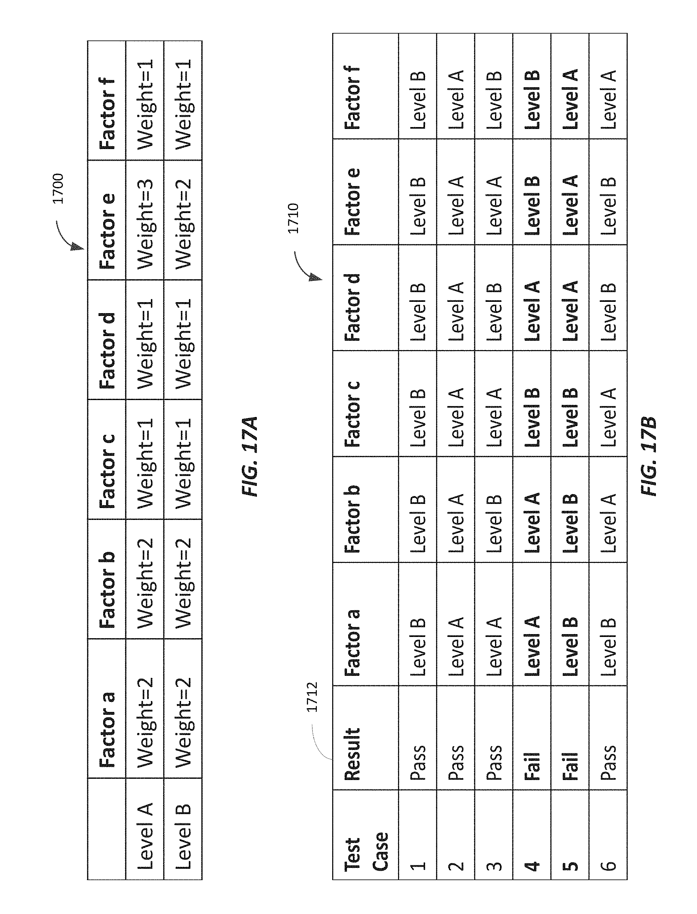
D00018
D00019

D00020

D00021

D00022

D00023
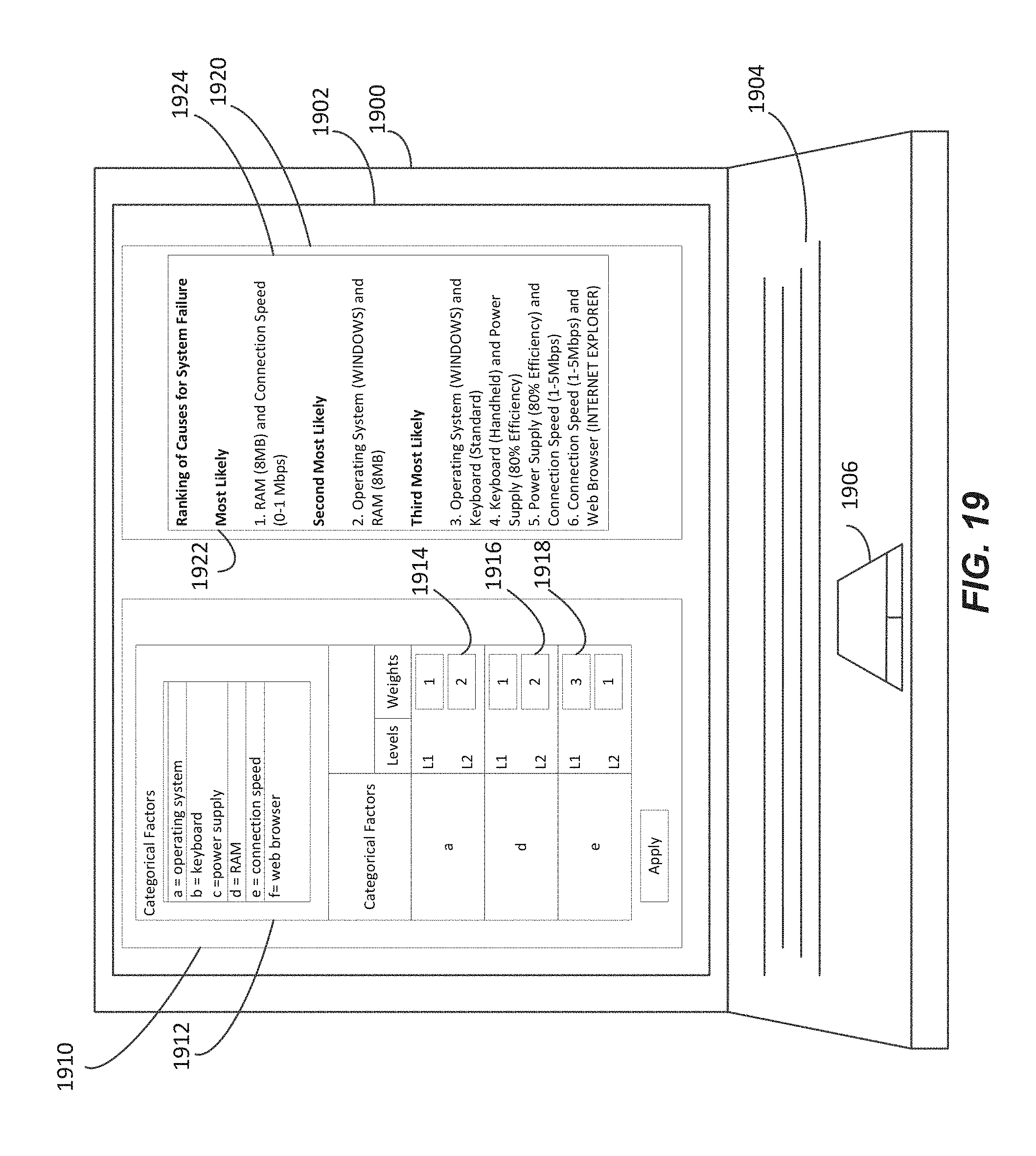
D00024

D00025

D00026

D00027

M00001

M00002

M00003

M00004

M00005

M00006

M00007

M00008

M00009

XML
uspto.report is an independent third-party trademark research tool that is not affiliated, endorsed, or sponsored by the United States Patent and Trademark Office (USPTO) or any other governmental organization. The information provided by uspto.report is based on publicly available data at the time of writing and is intended for informational purposes only.
While we strive to provide accurate and up-to-date information, we do not guarantee the accuracy, completeness, reliability, or suitability of the information displayed on this site. The use of this site is at your own risk. Any reliance you place on such information is therefore strictly at your own risk.
All official trademark data, including owner information, should be verified by visiting the official USPTO website at www.uspto.gov. This site is not intended to replace professional legal advice and should not be used as a substitute for consulting with a legal professional who is knowledgeable about trademark law.