Method For Multi-dimensional Identification Of Flexible Load Demand Response Effect
LIU; Dunnan ; et al.
U.S. patent application number 16/989511 was filed with the patent office on 2021-02-25 for method for multi-dimensional identification of flexible load demand response effect. The applicant listed for this patent is NORTH CHINA ELECTRIC POWER UNIVERSITY. Invention is credited to Zhi CAI, Changyou FENG, Rui GE, Jinshan HAN, Yiding JIN, Pengfei LI, Dunnan LIU, Jiangyan LIU, Da SONG, Nan WANG, Xingkai WANG, Zhao ZHAO.
| Application Number | 20210056647 16/989511 |
| Document ID | / |
| Family ID | 1000005050937 |
| Filed Date | 2021-02-25 |


View All Diagrams
| United States Patent Application | 20210056647 |
| Kind Code | A1 |
| LIU; Dunnan ; et al. | February 25, 2021 |
METHOD FOR MULTI-DIMENSIONAL IDENTIFICATION OF FLEXIBLE LOAD DEMAND RESPONSE EFFECT
Abstract
A method for multi-dimensional identification of flexible load demand response effects, including: step 1. determining a target object, a target area and a demand response project that participate in the multi-dimensional identification of flexible load demand response effects; step 2. acquiring flexible load evaluation data of the target area and the target object; step 3. performing data cleaning; step 4. preprocessing the flexible load evaluation data; step 5. constructing four characteristic extraction indicators, a peak load reduction rate, a peak-to-valley difference ratio, a load factor ratio and a response status, inputting a predicted value and an actual collected value of maximum and minimum daily loads before and after the flexible load demand response that are obtained from the prepossessing, to generate a matrix for clustering; step 6. clustering the matrix for clustering generated in step 5; step 7. guiding a more targeted development of demand response projects.
| Inventors: | LIU; Dunnan; (Beijing, CN) ; LI; Pengfei; (Beijing, CN) ; GE; Rui; (Beijing, CN) ; WANG; Xingkai; (Beijing, CN) ; CAI; Zhi; (Beijing, CN) ; JIN; Yiding; (Beijing, CN) ; FENG; Changyou; (Beijing, CN) ; ZHAO; Zhao; (Beijing, CN) ; WANG; Nan; (Beijing, CN) ; SONG; Da; (Beijing, CN) ; LIU; Jiangyan; (Beijing, CN) ; HAN; Jinshan; (Beijing, CN) | ||||||||||
| Applicant: |
|
||||||||||
|---|---|---|---|---|---|---|---|---|---|---|---|
| Family ID: | 1000005050937 | ||||||||||
| Appl. No.: | 16/989511 | ||||||||||
| Filed: | August 10, 2020 |
| Current U.S. Class: | 1/1 |
| Current CPC Class: | G06Q 30/0205 20130101; G06F 16/2365 20190101; G06Q 10/06375 20130101; G06Q 10/06313 20130101; G06Q 10/06315 20130101; H02J 13/00002 20200101; G05B 13/028 20130101; G06Q 50/06 20130101 |
| International Class: | G06Q 50/06 20060101 G06Q050/06; G06F 16/23 20060101 G06F016/23; G06Q 30/02 20060101 G06Q030/02; G06Q 10/06 20060101 G06Q010/06; G05B 13/02 20060101 G05B013/02; H02J 13/00 20060101 H02J013/00 |
Foreign Application Data
| Date | Code | Application Number |
|---|---|---|
| Aug 23, 2019 | CN | 201910785597. 8 |
Claims
1. A method for multi-dimensional identification of flexible load demand response effects, comprising: Step 1. determining a target object, a target area and a demand response project that participate in the multi-dimensional identification of flexible load demand response effects; Step 2. acquiring flexible load evaluation data of the target area and the target object in step 1; Step 3. performing data cleaning on the flexible load evaluation data acquired in step 2; Step 4. preprocessing the flexible load evaluation data after the cleaning in step 3, to obtain a predicted value and an actual collected value of maximum and minimum daily loads respectively before and after the flexible load demand response; Step 5. constructing four characteristic extraction indicators, a peak load reduction rate, a peak-to-valley difference ratio, a load factor ratio and a response status, inputting the predicted value and the actual collected value of maximum and minimum daily loads before and after the flexible load demand response that are obtained from the prepossessing in step 4, to generate a matrix for clustering; Step 6. clustering the matrix for clustering generated in step 5; Step 7. analyzing response characteristics corresponding to different classes based on the clustering result obtained in step 6 and the classes of flexible load demand responses obtained from the clustering, to guide a more targeted development of demand response projects.
2. The method for multi-dimensional identification of flexible load demand response effects according to claim 1, wherein step 1 comprises: (1) determining a target user group and typical users to participate in the evaluation: selecting a corresponding flexible load and determining an evaluation area; (2) determining a demand response project to participate in the evaluation, which includes time-of-use pricing, critical peak pricing, real-time pricing, ordered electricity consumption, interruptible load and direct load control.
3. The method for multi-dimensional identification of flexible load demand response effects according to claim 1, wherein step 2 comprises: acquiring 96-point historical daily load data before a demand response is implemented and 96-point flexible load data after the demand response is implemented for different types of flexible loads from an electricity usage collection system.
4. The method for multi-dimensional identification of flexible load demand response effects according to claim 1, wherein step 3 comprises: identifying and correcting identifiable errors in the data file by performing consistency checks and processing of missing and invalid values on the data.
5. The method for multi-dimensional identification of flexible load demand response effects according to claim 1, wherein step 4 comprises: (1) predicting a maximum value q.sub.max.sup.k' and a minimum value q.sub.min.sup.k' of a would-have-been flexible load during the period of the demand response based on the historical data of the flexible load, which comprises the following steps: {circle around (1)} calculating a yearly load growth rate r, according to the formula below: r = ( Q n - Q 1 Q 1 ) ( n - 1 ) - 1 ( 1 ) ##EQU00009## where r is the yearly load growth rate, n is the year, Q.sub.n is a total load in the nth year, and Q.sub.1 is a total load in the first year; {circle around (2)} predicting 96-point load data during the implementation of the demand response project based on the historical load growth rate r, according to the formula below: q.sub.n+1.sup.k',s=q.sub.n.sup.k,s.times.(1+r) (2) where n is the year, k is the kth day, s is the sth point in time, q.sub.n.sup.k,s is an actual load at the sth point on the kth day of the nth year, and q.sub.n+1.sup.k',s is a predicted load at the sth point on the kth day of the (n+1)th year; {circle around (3)} identifying maximum and minimum values q.sub.max.sup.k'={q.sub.max.sup.1', q.sub.max.sup.2', q.sub.max.sup.3' . . . }, q.sub.min.sup.k'={q.sub.min.sup.1', q.sub.min.sup.2', q.sub.min.sup.3'. . . }, q.sub.ave.sup.k'={q.sub.ave.sup.1', q.sub.ave.sup.2', q.sub.ave.sup.3' . . . } from the predicted 96-point load on the kth day of the period of the demand response, where k denotes the kth day, q.sub.max.sup.k' denotes a maximum value of the predicted 96-point load on the kth day, and q.sub.max.sup.k' d denotes a minimum value of the predicted 96-point load on the kth day; (2) identifying and acquiring maximum and minimum values, q.sub.max.sup.k={q.sub.max.sup.1, q.sub.max.sup.2, q.sub.max.sup.3 . . . }, q.sub.min.sup.k={q.sub.min.sup.1, q.sub.min.sup.2, q.sub.min.sup.3 . . . }, an average value q.sub.ave.sup.k={q.sub.ave.sup.1, q.sub.ave.sup.2, q.sub.ave.sup.3 . . . } of the load in every k days based on the collected 96-point load data during the actual demand response, where k denotes the kth day, q.sub.max.sup.k denotes a maximum value of the 96-point load on the kth day that is actually collected, and q.sub.min.sup.k denotes a minimum value of the 96-point load on the kth day that is actually collected.
6. The method for multi-dimensional identification of flexible load demand response effects according to claim 1, wherein step 5 comprises: (1) extracting four flexible load characteristic indicators, a peak load reduction rate, a peak-to-valley difference ratio, a load factor ratio and a response status: {circle around (1)} Peak load reduction rate: PR.sup.k=(q.sub.max.sup.k'-q.sub.max.sup.k)/q.sub.max.sup.k'.times.100% (3) where PR.sup.k is a peak load reduction rate on the kth day, and q.sub.max.sup.k' and q.sub.max.sup.k are peak loads before and after the flexible load response on the kth day respectively; {circle around (2)} Peak-to-valley difference ratio: PtV.sup.k=(q.sub.max.sup.k'-q.sub.min.sup.k')/(q.sub.max.sup.k-q.sub.min.- sup.k).times.100% (4) where PtV.sup.k is a peak-to-valley difference ratio on the kth day, and q.sub.max.sup.k' and q.sub.max.sup.k are peak loads before and after the flexible load response on the kth day respectively; {circle around (3)} Load factor ratio: LF k = q ave k ' q max k ' .times. q max k q ave k .times. 100 % ( 5 ) ##EQU00010## where LF.sup.k is a load factor rate on the kth day, q.sub.max.sup.k is peak load before and after the flexible load response on the kth day, and q.sub.ave.sup.k is an average value of the flexible load on the kth day; {circle around (4)} Response status: RS k = { 1 , PR k > .alpha. 0 , PR k .ltoreq. .alpha. ( 6 ) ##EQU00011## where RS.sup.k is a response status on the kth day, PR.sup.k is the peak load reduction rate on the kth day, and .alpha. is a predetermined threshold for the peak load reduction rate; .alpha. is used to determine whether or not to respond: 1 indicates response while 0 indicates non-response; (2) generating a matrix for clustering from the four flexible load characteristic indicators according to the four flexible load characteristic indicators, peak load reduction rate, peak-to-valley difference ratio, load factor ratio and response status, and (2) of step 5 specifically comprising: {circle around (1)} taking four characteristic indicators calculated from a user daily as one sample, so that the user i has a matrix for clustering, Y.sub.L.times.4, that represents a load curve characteristic indicator; {circle around (2)} with Y.sub.L.times.4 being an input, clustering by using Euclidean distance as a similarity criterion, where L is the duration of the demand response, "4" denotes the number of indicators, and Y.sub.L.times.4 is the matrix for clustering.
7. The method for multi-dimensional identification of flexible load demand response effects according to claim 1, wherein step 6 comprises: (1) repeatedly selecting a cluster center to perform a clustering with the number of clusters being k: {circle around (1)} determining the number of clusters k to range from k.sub.min=2 to k.sub.max=int( {square root over (x)}), where s denotes the number of samples; {circle around (2)} calculating the distance between each sample and an initial cluster center, and classifying the samples into clusters that minimize the distance; {circle around (3)} recalculating each cluster center, recalculating the distance, the classification and the cluster center until the number of iterations is reached or the distances within the clusters can no longer be reduced, thereby completing the clustering with the number of clusters being k; (2) assessing and optimizing the clustering result in (1) of step 6 by using a Silhouette index for calculating the effectiveness of clustering, and determining final number of clusters, clustering result and cluster center: {circle around (1)} with a (x) being an average distance between a sample x in cluster C.sub.j and all the other samples in the cluster to represent the degree of tightness within the cluster, with d (x, C.sub.i) being an average distance between the sample x and all samples in another cluster C.sub.i, with b (x) being a minimum average distance between the sample x and all samples outside the same cluster as x, to represent the degree of dispersion between clusters, b (x)=min {d (x, Ci)}, i=1, 2, . . . , k, i.noteq.j; calculating a Silhouette index for each sample x according to equation (7): S ( x ) = b ( x ) - a ( x ) min { a ( x ) , b ( x ) } ( 7 ) ##EQU00012## where b (x) is the minimum average distance between the sample x and all samples outside the same cluster as x, and a (x) is the average distance between the sample x in cluster C.sub.j and all the other samples in the cluster; {circle around (2)} obtaining a clustering result and a cluster center from the four flexible load four characteristic indicators, after the optimization of the Silhouette index.
8. The method for multi-dimensional identification of flexible load demand response effects according to claim 1, wherein step 7 comprises: (1) analyzing response capacity, response speed, response period of each class of flexible load and demand response effects of different demand response projects according to the classification result of different flexible loads from step 6: {circle around (1)} the magnitude of the peak load reduction rate indicates peak-cutting capability in electricity consumption peak hours; {circle around (2)} the magnitude of the peak-to-valley difference ratio and the magnitude of the load ratio indicate peak cutting and valley filling capabilities of a user; {circle around (3)} The transition speed of the response status from 0 to 1 indicates response speed of a user demand response project; (2) developing demand response projects in a more targeted manner based on the analysis of the user demand response effects in (1) of step 7: {circle around (1)} If a demand response project requires cutting a peak power load, developing the demand response project mainly for users with a large peak load reduction rate; {circle around (2)} If a demand response project requires smoothing an electricity usage curve and alleviating peak scheduling of a power grid, developing the demand response project mainly for users with a stable load ratio and a large peak-to-valley difference ratio; {circle around (3)} If a demand response project requires quick response, developing the demand response project mainly for users with a fast response speed in the response status; {circle around (4)} If a demand response project requires continuous response, developing the demand response project mainly for users with a long response period in the response status.
Description
TECHNICAL FIELD
[0001] The present disclosure relates to the technical field of demand-side power management, and to a method for identification of demand response effects, in particular to a method for multi-dimensional identification of flexible load demand response effects.
BACKGROUND
[0002] Flexible load refers to electricity consumption changing within a specified interval or moving around between different periods, including adjustable or transferable loads with demand flexibility, and electric vehicles, energy storages, distributed power supplies and microgrids with two-way adjustment capability.
[0003] Demand response refers to a variety of short-term behaviors of electricity users to actively adjust the way they use electricity in accordance with electricity price changes and incentive policies. Generally, flexible load is regulated and scheduled by demand response projects. Flexible load scheduling, as a supplement to power generation scheduling, can cut peaks and fill valleys, balance intermittent energy fluctuations and provide auxiliary functions, and thus is a regulative measure that facilities power grid scheduling operations. Identifying the effect of flexible load participation in demand response is of great significance for flexible load scheduling, and can guide the development of demand response projects and enable a more targeted development of demand response projects.
[0004] However, most of the existing researches and technologies have focused on identifying and analyzing the potential of flexible load in demand response, mainly used to estimate the effect of demand response projects before they are launched. What lacks is a method to analyze the actual effect of flexible load participation in demand response. The analysis of the actual effect of flexible load participating in demand response is particularly important for flexible load scheduling and for understanding development effects of demand response projects. With the gradual advancement of China's demand response projects, the method for analyzing flexible load demand response effects will play an increasingly important role.
SUMMARY OF PARTICULAR EMBODIMENTS
[0005] An object of the present disclosure is to overcome the drawbacks in the prior art, and to provide a method for multi-dimensional identification of flexible load demand response effects.
[0006] The present disclosure solves the technical problems by the following technical solutions:
[0007] A method for multi-dimensional identification of flexible load demand response effects, including the following steps:
[0008] Step 1. determining a target object, a target area and a demand response project that participate in the multi-dimensional identification of flexible load demand response effects;
[0009] Step 2. acquiring flexible load evaluation data of the target area and the target object in step 1;
[0010] Step 3. performing data cleaning on the flexible load evaluation data acquired in step 2;
[0011] Step 4. preprocessing the flexible load evaluation data after the cleaning in step 3, to obtain a predicted value and an actual collected value of maximum and minimum daily loads respectively before and after the flexible load demand response;
[0012] Step 5. constructing four characteristic extraction indicators, a peak load reduction rate, a peak-to-valley difference ratio, a load factor ratio and a response status, inputting the predicted value and the actual collected value of maximum and minimum daily loads before and after the flexible load demand response that are obtained from the prepossessing in step 4, to generate a matrix for clustering;
[0013] Step 6. clustering the matrix for clustering generated in step 5;
[0014] Step 7. analyzing response characteristics corresponding to different classes based on the clustering result obtained in step 6 and the classes of flexible load demand responses obtained from the clustering, to guide a more targeted development of demand response projects.
[0015] Specifically, step 1 includes:
[0016] (1) determining a target user group and typical users to participate in the evaluation: selecting a corresponding flexible load and determining an evaluation area;
[0017] (2) determining a demand response project to participate in the evaluation, which includes time-of-use pricing, critical peak pricing, real-time pricing, ordered electricity consumption, interruptible load and direct load control.
[0018] Specifically, step 2 includes:
[0019] acquiring 96-point historical daily load data before a demand response is implemented and 96-point flexible load data after the demand response is implemented for different types of flexible loads from an electricity usage collection system.
[0020] Specifically, step 3 includes:
[0021] identifying and correcting identifiable errors in the data file by performing consistency checks and processing of missing and invalid values on the data.
[0022] Specifically, step 4 includes:
[0023] (1) predicting a maximum value q.sub.max.sup.k' and a minimum value q.sub.min.sup.k' of a would-have-been flexible load during the period of the demand response based on the historical data of the flexible load, which comprises the following steps:
[0024] {circle around (1)} calculating a yearly load growth rate r, according to the formula below:
r = ( Q n - Q 1 Q 1 ) ( n - 1 ) - 1 ( 1 ) ##EQU00001##
[0025] where r is the yearly load growth rate, n is the year, Q.sub.n is a total load in the nth year, and Q.sub.1 is a total load in the first year;
[0026] {circle around (2)} predicting 96-point load data during the implementation of the demand response project based on the historical load growth rate r, according to the formula below:
q.sub.n+1.sup.k',s=q.sub.n.sup.k,s.times.(1+r) (2)
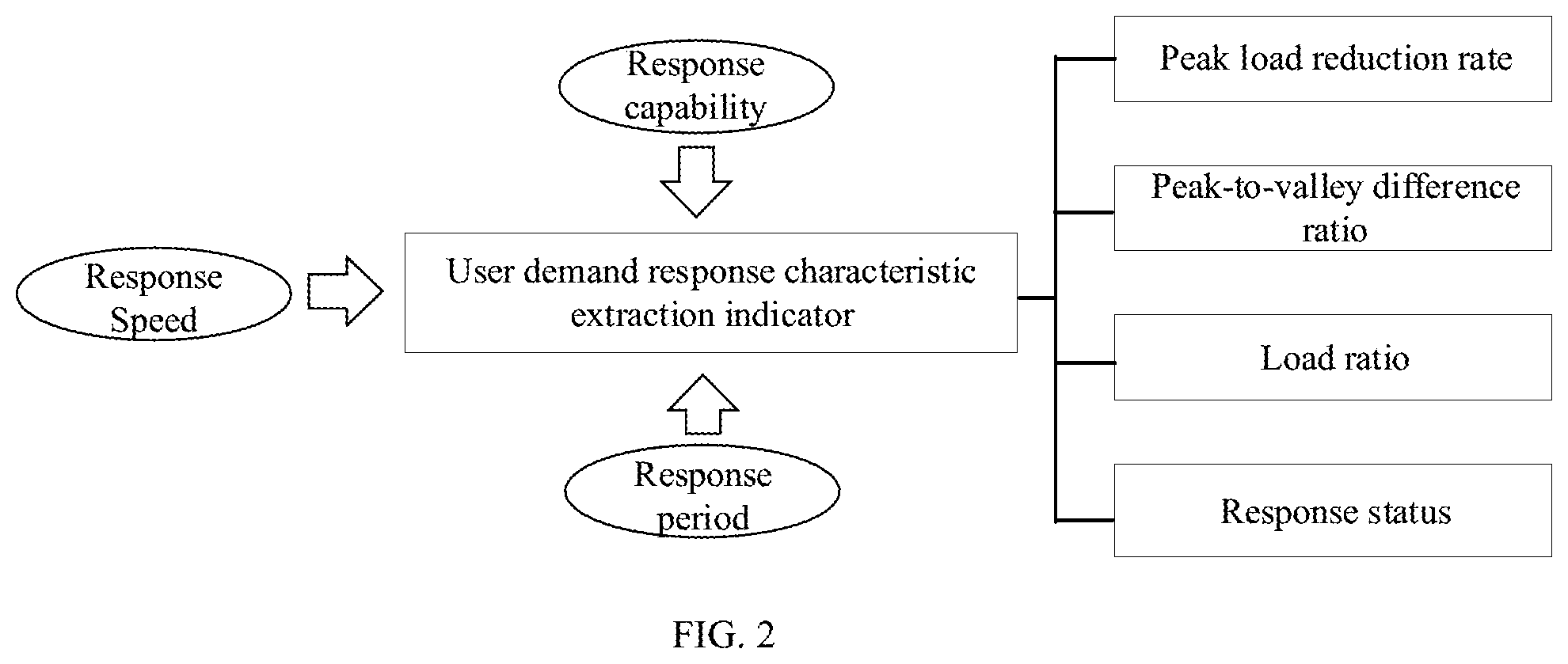
[0027] where n is the year, k is the kth day, s is the sth point in time, q.sub.n.sup.k,s is an actual load at the sth point on the kth day of the nth year, and q.sub.n+1.sup.k',s is a predicted load at the sth point on the kth day of the (n+1)th year;
[0028] {circle around (3)} identifying maximum and minimum values q.sub.max.sup.k'={q.sub.max.sup.1', q.sub.max.sup.2', q.sub.max.sup.3' . . . }, q.sub.min.sup.k'={q.sub.min.sup.1', q.sub.min.sup.2', q.sub.min.sup.3'. . . }, q.sub.ave.sup.k'={q.sub.ave.sup.1', q.sub.ave.sup.2', q.sub.ave.sup.3', . . . } from the predicted 96-point load on the kth day of the period of the demand response,
[0029] where k denotes the kth day, q.sub.max.sup.k' denotes a maximum value of the predicted 96-point load on the kth day, and q.sub.min.sup.k' denotes a minimum value of the predicted 96-point load on the kth day;
[0030] (2) identifying and acquiring maximum and minimum values, q.sub.max.sup.k={q.sub.max.sup.1, q.sub.max.sup.2, q.sub.max.sup.3 . . . }, q.sub.min.sup.k={q.sub.min.sup.1, q.sub.min.sup.2, q.sub.min.sup.3 . . . }, an average value q.sub.ave.sup.k={q.sub.ave.sup.1, q.sub.ave.sup.2, q.sub.ave.sup.3 . . . } of the load in every k days based on the collected 96-point load data during the actual demand response,
[0031] where k denotes the kth day, q.sub.max.sup.k denotes a maximum value of the 96-point load on the kth day that is actually collected, and q.sub.min.sup.k denotes a minimum value of the 96-point load on the kth day that is actually collected.
[0032] Specifically, step 5 includes:
[0033] (1) extracting four flexible load characteristic indicators, a peak load reduction rate, a peak-to-valley difference ratio, a load factor ratio and a response status:
[0034] {circle around (1)} Peak load reduction rate:
PR.sup.k=(q.sub.max.sup.k'-q.sub.max.sup.k)/q.sub.max.sup.k'.times.100% (3)
[0035] where PR.sup.k is a peak load reduction rate on the kth day, and q.sub.max.sup.k' and q.sub.max.sup.k are peak loads before and after the flexible load response on the kth day respectively;
[0036] {circle around (2)} Peak-to-valley difference ratio:
PtV.sup.k=(q.sub.max.sup.k'-q.sub.min.sup.k')/(q.sub.max.sup.k-q.sub.min- .sup.k).times.100% (4)
[0037] where PtV.sup.k is a peak-to-valley difference ratio on the kth day, and q.sub.max.sup.k' and q.sub.max.sup.k are peak loads before and after the flexible load response on the kth day respectively;
[0038] {circle around (3)} Load factor ratio:
LF k = q ave k ' q max k ' .times. q max k q ave k .times. 100 % ( 5 ) ##EQU00002##
[0039] where LF.sup.k is a load factor rate on the kth day, q.sub.max.sup.k is peak load before and after the flexible load response on the kth day, and q.sub.ave.sup.k is an average value of the flexible load on the kth day;
[0040] {circle around (4)} Response status:
RS k = { 1 , PR k > .alpha. 0 , PR k .ltoreq. .alpha. ( 6 ) ##EQU00003##
[0041] where RS.sup.k is a response status on the kth day, PR.sup.k is the peak load reduction rate on the kth day, and .alpha. is a predetermined threshold for the peak load reduction rate; .alpha. is used to determine whether or not to respond: 1 indicates response while 0 indicates non-response;
[0042] (2) generating a matrix for clustering from the four flexible load characteristic indicators according to the four flexible load characteristic indicators, peak load reduction rate, peak-to-valley difference ratio, load factor ratio and response status, and
[0043] (2) of step 5 specifically comprising:
[0044] {circle around (1)} taking four characteristic indicators calculated from a user daily as one sample, so that the user i has a matrix for clustering, Y.sub.L.times.4, that represents a load curve characteristic indicator;
[0045] {circle around (2)} with Y.sub.L.times.4 being an input, clustering by using Euclidean distance as a similarity criterion,
[0046] where L is the duration of the demand response, "4" denotes the number of indicators, and Y.sub.L.times.4 is the matrix for clustering.
[0047] Specifically, step 6 includes:
[0048] (1) repeatedly selecting a cluster center to perform a clustering with the number of clusters being k:
[0049] {circle around (1)} determining the number of clusters k to range from k.sub.min=2 to k.sub.max=int( {square root over (x)}) where s denotes the number of samples;
[0050] {circle around (2)} calculating the distance between each sample and an initial cluster center, and classifying the samples into clusters that minimize the distance;
[0051] {circle around (3)} recalculating each cluster center, recalculating the distance, the classification and the cluster center until the number of iterations is reached or the distances within the clusters can no longer be reduced, thereby completing the clustering with the number of clusters being k;
[0052] (2) assessing and optimizing the clustering result in (1) of step 6 by using a Silhouette index for calculating the effectiveness of clustering, and determining final number of clusters, clustering result and cluster center:
[0053] {circle around (1)} with a (x) being an average distance between a sample x in cluster C.sub.j and all the other samples in the cluster to represent the degree of tightness within the cluster, with d (x, C.sub.i) being an average distance between the sample x and all samples in another cluster C.sub.i, with b (x) being a minimum average distance between the sample x and all samples outside the same cluster as x, to represent the degree of dispersion between clusters, b (x)=min{d(x, Ci)}, i=1, 2, . . . , k, i.noteq.j;
[0054] calculating a Silhouette index for each sample x according to equation (7):
S ( x ) = b ( x ) - a ( x ) min { a ( x ) , b ( x ) } ( 7 ) ##EQU00004##
[0055] where b (x) is the minimum average distance between the sample x and all samples outside the same cluster as x, and a (x) is the average distance between the sample x in cluster C.sub.j and all the other samples in the cluster;
[0056] {circle around (2)} obtaining a clustering result and a cluster center from the four flexible load four characteristic indicators, after the optimization of the Silhouette index.
[0057] Specifically, step 7 includes:
[0058] (1) analyzing response capacity, response speed, response period of each class of flexible load and demand response effects of different demand response projects according to the classification result of different flexible loads from step 6:
[0059] {circle around (1)} the magnitude of the peak load reduction rate indicates peak-cutting capability in electricity consumption peak hours;
[0060] {circle around (2)} the magnitude of the peak-to-valley difference ratio and the magnitude of the load ratio indicate peak cutting and valley filling capabilities of a user;
[0061] {circle around (3)} The transition speed of the response status from 0 to 1 indicates response speed of a user demand response project;
[0062] (2) developing demand response projects in a more targeted manner based on the analysis of the user demand response effects in (1) of step 7:
[0063] {circle around (1)} If a demand response project requires cutting a peak power load, developing the demand response project mainly for users with a large peak load reduction rate;
[0064] {circle around (2)} If a demand response project requires smoothing an electricity usage curve and alleviating peak scheduling of a power grid, developing the demand response project mainly for users with a stable load ratio and a large peak-to-valley difference ratio;
[0065] {circle around (3)} If a demand response project requires quick response, developing the demand response project mainly for users with a fast response speed in the response status;
[0066] {circle around (4)} If a demand response project requires continuous response, developing the demand response project mainly for users with a long response period in the response status.
[0067] The present disclosure has the following advantages and positive effects:
[0068] Upon preprocessing flexible load data collected by an electricity usage collecting device, based on four extracted characteristic indicators, a peak load reduction rate, a peak-to-valley difference ratio, a load factor ratio and a response status, the present disclosure extracts flexible load demand response characteristics relatively comprehensively from the aspects of response capacity, response speed and response period, and compares the actual load status with a predicted load status, to scientifically reflect the actual effect of flexible load demand response. Then, the flexible load demand response characteristics are appropriately classified and identified, and demand response projects are developed in a more targeted manner in accordance with the different classes of response characteristics, to achieve such purposes as: when peak cutting, valley filling, rapid demand response or continuous demand response is needed, target users can be discovered so that a more effective flexible load scheduling and demand response project development can be realized.
BRIEF DESCRIPTION OF THE DRAWINGS
[0069] FIG. 1 is a flowchart of a method for multi-dimensional identification of flexible load demand response effects based on collected electricity usage data according to the present disclosure;
[0070] FIG. 2 is a schematic diagram of an indicator for multi-dimensional identification of flexible load demand response effects according to the present disclosure.
DETAILED DESCRIPTION OF PARTICULAR EMBODIMENTS
[0071] The embodiments of the present disclosure will be described in detail below with reference to the accompanying drawings.
[0072] As shown in FIG. 1 and FIG. 2, a method for multi-dimensional identification of flexible load demand response effects includes the following steps:
[0073] Step 1. determining a target object, a target area and a demand response project that participate in the multi-dimensional identification of flexible load demand response effects.
[0074] Specifically, step 1 includes:
[0075] (1) determining a target user group and typical users to participate in the evaluation: selecting a corresponding flexible load and determining an evaluation area;
[0076] (2) determining a demand response project to participate in the evaluation, which includes time-of-use pricing, critical peak pricing, real-time pricing, ordered electricity consumption, interruptible load and direct load control.
[0077] Step 2. acquiring flexible load evaluation data of the target area and the target object in step 1.
[0078] Specifically, step 2 includes:
[0079] acquiring 96-point historical daily load data before a demand response is implemented and 96-point flexible load data after the demand response is implemented for different types of flexible loads from an electricity usage collection system.
[0080] Step 3. performing data cleaning on the flexible load evaluation data acquired in step 2.
[0081] Specifically, step 3 includes:
[0082] identifying and correcting identifiable errors in the data file by performing consistency checks and processing of missing and invalid values on the data.
[0083] Step 4. preprocessing the flexible load evaluation data after the cleaning in step 3, to obtain a predicted value and an actual collected value of maximum and minimum daily loads respectively before and after the flexible load demand response;
[0084] predicting normal daily load data corresponding to the period of the demand response based on historical daily load data, and extracting the maximum and minimum daily loads before and after the flexible load demand response according to actual data from the implemented demand response project.
[0085] Specifically, step 4 includes:
[0086] (1) predicting a maximum value q.sub.max.sup.k' and a minimum value q.sub.min.sup.k' of a would-have-been flexible load during the period of the demand response based on the historical data of the flexible load, which includes the following steps:
[0087] {circle around (1)} calculating a yearly load growth rate r, according to the formula below:
r = ( Q n - Q 1 Q 1 ) ( n - 1 ) - 1 ( 1 ) ##EQU00005##
[0088] where r is the yearly load growth rate, n is the year, Q.sub.n is a total load in the nth year, and Q.sub.1 is a total load in the first year;
[0089] {circle around (2)} predicting 96-point load data during the implementation of the demand response project based on the historical load growth rate r, according to the formula below:
q.sub.n+1.sup.k',s=q.sub.n.sup.k,s.times.(1+r) (2)
[0090] where n is the year, k is the kth day, s is the sth point in time, q.sub.n.sup.k,s is an actual load at the sth point on the kth day of the nth year, and q.sub.n+1.sup.k',s is a predicted load at the sth point on the kth day of the (n+1)th year;
[0091] {circle around (3)} identifying maximum and minimum values q.sub.max.sup.k'={q.sub.max.sup.1', q.sub.max.sup.2', q.sub.max.sup.3'. . . }, q.sub.min.sup.k'={q.sub.min.sup.1', q.sub.min.sup.2', q.sub.min.sup.3'. . . }, ={q.sub.ave.sup.1', q.sub.ave.sup.2', q.sub.ave.sup.3' . . . } from the predicted 96-point load on the kth day of the period of the demand response,
[0092] where k denotes the kth day, q.sub.max.sup.k' denotes a maximum value of the predicted 96-point load on the kth day, and q.sub.min.sup.k' denotes a minimum value of the predicted 96-point load on the kth day.
[0093] (2) identifying and acquiring maximum and minimum values, q.sub.max.sup.k={q.sub.max.sup.1, q.sub.max.sup.2, q.sub.max.sup.3 . . . }, q.sub.min.sup.k={q.sub.min.sup.1, q.sub.min.sup.2, q.sub.min.sup.3 . . . }, an average value q.sub.ave.sup.k={q.sub.ave.sup.1, q.sub.ave.sup.2, q.sub.ave.sup.3 . . . } of the load in every k days based on the collected 96-point load data during the actual demand response,
[0094] where k denotes the kth day, q.sub.max.sup.k denotes a maximum value of the 96-point load on the kth day that is actually collected, and q.sub.min.sup.k denotes a minimum value of the 96-point load on the kth day that is actually collected.
[0095] Step 5. constructing four characteristic extraction indicators, a peak load reduction rate, a peak-to-valley difference ratio, a load factor ratio and a response status, inputting the predicted value and the actual collected value of maximum and minimum daily loads before and after the flexible load demand response that are obtained from the prepossessing in step 4, to generate a matrix for clustering;
[0096] generating a matrix for clustering according to predetermined characteristic extraction indicators, a peak load reduction rate, a peak-to-valley difference ratio, a load factor ratio and a response status, and by inputting the prepossessed data.
[0097] Specifically, step 5 includes:
[0098] (1) extracting four flexible load characteristic indicators, a peak load reduction rate, a peak-to-valley difference ratio, a load factor ratio and a response status:
[0099] {circle around (1)} Peak load reduction rate:
PR.sup.k=(q.sub.max.sup.k'-q.sub.max.sup.k)/q.sub.max.sup.k'.times.100% (3)
[0100] where PR.sup.k is a peak load reduction rate on the kth day, and q.sub.max.sup.k' and q.sub.max.sup.k are peak loads before and after the flexible load response on the kth day respectively;
[0101] {circle around (2)} Peak-to-valley difference ratio:
PtV.sup.k=(q.sub.max.sup.k'-q.sub.min.sup.k')/(q.sub.max.sup.k-q.sub.min- .sup.k).times.100% (4)
[0102] where PtV.sup.k is a peak-to-valley difference ratio on the kth day, and q.sub.max.sup.k' and q.sub.max.sup.k are peak loads before and after the flexible load response on the kth day respectively;
[0103] {circle around (3)} Load factor ratio:
LF k = q ave k ' q max k ' .times. q max k q ave k .times. 100 % ( 5 ) ##EQU00006##
[0104] where LF.sup.k is a load factor rate on the kth day, q.sub.max.sup.k is peak load before and after the flexible load response on the kth day, and q.sub.ave.sup.k is an average value of the flexible load on the kth day;
[0105] {circle around (4)} Response status:
RS k = { 1 , PR k > .alpha. 0 , PR k .ltoreq. .alpha. ( 6 ) ##EQU00007##
[0106] where RS.sup.k is a response status on the kth day, PR.sup.k is the peak load reduction rate on the kth day, and .alpha. is a predetermined threshold for the peak load reduction rate; .alpha. is used to determine whether or not to respond: 1 indicates response while 0 indicates non-response.
[0107] (2) generating a matrix for clustering from the four flexible load characteristic indicators according to the four flexible load characteristic indicators, peak load reduction rate, peak-to-valley difference ratio, load factor ratio and response status.
[0108] Specifically, (2) of step 5 includes:
[0109] {circle around (1)} taking four characteristic indicators calculated from a user daily as one sample, so that the user i has a matrix for clustering, Y.sub.L.times.4, that represents a load curve characteristic indicator;
[0110] {circle around (2)} with Y.sub.L.times.4 being an input, clustering by using Euclidean distance as a similarity criterion,
[0111] where L is the duration of the demand response, "4" denotes the number of indicators, and Y.sub.L.times.4 is the matrix for clustering.
[0112] Step 6. clustering by k-means clustering, based on the matrix for clustering generated in step 5;
[0113] k-means clustering the matrix for clustering, continuously modifying the number of clusters, and assessing a clustering result by using a Silhouette index.
[0114] (1) repeatedly selecting a cluster center to perform a clustering with the number of clusters being k;
[0115] {circle around (1)} determining the number of clusters k to range from k.sub.min=2 to k.sub.max=int( {square root over (x)}) where s denotes the number of samples;
[0116] {circle around (2)} calculating the distance between each sample and an initial cluster center, and classifying the samples into clusters that minimize the distance;
[0117] {circle around (3)} recalculating each cluster center, recalculating the distance, the classification and the cluster center until the number of iterations is reached or the distances within the clusters can no longer be reduced, thereby completing the clustering with the number of clusters being k.
[0118] (2) assessing and optimizing the clustering result in (1) of step 6 by using a Silhouette index for calculating the effectiveness of clustering, and determining final number of clusters, clustering result and cluster center;
[0119] {circle around (1)} with a (x) being an average distance between a sample x in cluster C.sub.j and all the other samples in the cluster to represent the degree of tightness within the cluster, with d (x, C.sub.i) being an average distance between the sample x and all samples in another cluster C.sub.i, with b (x) being a minimum average distance between the sample x and all samples outside the same cluster as x, to represent the degree of dispersion between clusters, b (x)=min{d(x, Ci)}, i=1, 2, . . . , k, i.noteq.j;
[0120] calculating a Silhouette index for each sample x according to equation (7):
S ( x ) = b ( x ) - a ( x ) min { a ( x ) , b ( x ) } ( 7 ) ##EQU00008##
[0121] where b (x) is the minimum average distance between the sample x and all samples outside the same cluster as x, and a (x) is the average distance between the sample x in cluster C.sub.j and all the other samples in the cluster;
[0122] The Silhouette index S (x) of the sample x varies within the range of [-1,1]; the smaller a (x) is, the larger b (x) is, the closer S (x) is to 1, and the better the within-cluster tightness and between-cluster dispersion of cluster j to which i belongs are; when a (x)>b (x), S (x)<0, and the distance between the sample x and samples outside the same cluster as x is smaller than the distance between the sample x and the samples in the cluster, which indicates the clustering fails; the larger the Silhouette index is, the better the clustering quality is; the maximum Silhouette index corresponds to the optimal number of clusters.
[0123] {circle around (2)} obtaining a clustering result and a cluster center from the four flexible load four characteristic indicators, after the optimization of the Silhouette index.
[0124] Step 7. analyzing response characteristics corresponding to different classes based on the clustering result obtained in step 6 and the classes of flexible load demand responses obtained from the clustering, to guide a more targeted development of demand response projects.
[0125] Specifically, step 7 includes:
[0126] (1) analyzing response capacity, response speed, response period of each class of flexible load and demand response effects of different demand response projects according to the classification result of different flexible loads from step 6.
[0127] {circle around (1)} the magnitude of the peak load reduction rate indicates peak-cutting capability in electricity consumption peak hours, i.e., the capability of reduction of the demand response. The greater the peak load reduction rate is, the greater the response capacity;
[0128] {circle around (2)} the magnitude of the peak-to-valley difference ratio and the magnitude of the load ratio indicate peak cutting and valley filling capabilities of a user. In the case where the load ratio does not vary largely, the greater the peak-to-valley difference ratio is, the stronger the peak cutting and valley filling capabilities of the user is.
[0129] {circle around (3)} The transition speed of the response status from 0 to 1 indicates response speed of a user demand response project, i.e., the length of time from when a user does not respond to when the user responds. The more the number of 1s in the response statuses, the longer the time the user responds, and the longer the response period is.
[0130] (2) developing demand response projects in a more targeted manner based on the analysis of the user demand response effects in (1) of step 7.
[0131] {circle around (1)} If a demand response project requires cutting a peak power load, developing the demand response project mainly for users with a large peak load reduction rate;
[0132] {circle around (2)} If a demand response project requires smoothing an electricity usage curve and alleviating peak scheduling of a power grid, developing the demand response project mainly for users with a stable load ratio and a large peak-to-valley difference ratio;
[0133] {circle around (3)} If a demand response project requires quick response, developing the demand response project mainly for users with a fast response speed in the response status;
[0134] {circle around (4)} If a demand response project requires continuous response, developing the demand response project mainly for users with a long response period in the response status.
[0135] The demand response project can also be designed and implemented for targeted users by synthetically considering various characteristics and needs.
[0136] From the calculation process above, it can be seen that this method synthetically considers such characteristics as response capacity, response speed and response period, relatively comprehensively measures the effects of flexible load demand response, compares the actual load status with a predicted load status, and can scientifically reflect the effect of flexible load demand response. The whole calculation process is clear-thinking and has a good applicability, making it suitable for wide application.
[0137] It should be noted that the embodiments described herein are for illustrative purposes only and shall not be construed as limiting the scope of the present invention. Therefore, those embodiments made by the skilled in the art based on the embodiments described herein shall fall within the scope of the present invention.
* * * * *
D00000
D00001
D00002


XML
uspto.report is an independent third-party trademark research tool that is not affiliated, endorsed, or sponsored by the United States Patent and Trademark Office (USPTO) or any other governmental organization. The information provided by uspto.report is based on publicly available data at the time of writing and is intended for informational purposes only.
While we strive to provide accurate and up-to-date information, we do not guarantee the accuracy, completeness, reliability, or suitability of the information displayed on this site. The use of this site is at your own risk. Any reliance you place on such information is therefore strictly at your own risk.
All official trademark data, including owner information, should be verified by visiting the official USPTO website at www.uspto.gov. This site is not intended to replace professional legal advice and should not be used as a substitute for consulting with a legal professional who is knowledgeable about trademark law.