Systems And Methods For Modeling Noise Sequences And Calibrating Quantum Processors
Raymond; Jack R.
U.S. patent application number 16/878364 was filed with the patent office on 2020-12-03 for systems and methods for modeling noise sequences and calibrating quantum processors. The applicant listed for this patent is D-WAVE SYSTEMS INC.. Invention is credited to Jack R. Raymond.
| Application Number | 20200380396 16/878364 |
| Document ID | / |
| Family ID | 1000004867573 |
| Filed Date | 2020-12-03 |


| United States Patent Application | 20200380396 |
| Kind Code | A1 |
| Raymond; Jack R. | December 3, 2020 |
SYSTEMS AND METHODS FOR MODELING NOISE SEQUENCES AND CALIBRATING QUANTUM PROCESSORS
Abstract
Calibration techniques for devices of analog processors to remove time-dependent biases are described. Devices in an analog processor exhibit a noise spectrum that spans a wide range of frequencies, characterized by 1/f spectrum. Offset parameters are determined assuming only a given power spectral density. The algorithm determines a model for a measurable quantity of a device in an analog processor associated with a noise process and an offset parameter, determines the form of the spectral density of the noise process, approximates the noise spectrum by a discrete distribution via the digital processor, constructs a probability distribution of the noise process based on the discrete distribution and evaluates the probability distribution to determine optimized parameter settings to enhance computational efficiency.
| Inventors: | Raymond; Jack R.; (Vancouver, CA) | ||||||||||
| Applicant: |
|
||||||||||
|---|---|---|---|---|---|---|---|---|---|---|---|
| Family ID: | 1000004867573 | ||||||||||
| Appl. No.: | 16/878364 | ||||||||||
| Filed: | May 19, 2020 |
Related U.S. Patent Documents
| Application Number | Filing Date | Patent Number | ||
|---|---|---|---|---|
| 62855512 | May 31, 2019 | |||
| Current U.S. Class: | 1/1 |
| Current CPC Class: | G01R 29/26 20130101; G06N 10/00 20190101; G06N 7/005 20130101; B82Y 35/00 20130101; G01R 33/24 20130101 |
| International Class: | G06N 7/00 20060101 G06N007/00; G06N 10/00 20060101 G06N010/00; G01R 29/26 20060101 G01R029/26; G01R 33/24 20060101 G01R033/24 |
Claims
1. A method of operation of a hybrid processor, the hybrid processor comprising an analog processor and a digital processor, the analog processor having a plurality of devices, at least one of the plurality of devices having a measurable quantity associated with a noise process and an offset parameter, the method comprising: receiving by the digital processor a model for the measurable quantity and a form of a spectral density of the noise process; approximating a noise spectrum of the noise process by a discrete distribution via the digital processor; constructing a probability distribution of the noise process based on the discrete distribution via the digital processor; and evaluating the probability distribution to determine a number of optimized parameter settings via the digital processor.
2. The method of claim 1, further comprising: applying the optimized parameter settings to one or more of the plurality of devices of the analog processor to at least partially compensate for the noise process over time.
3. The method of claim 1 wherein receiving by the digital processor a model for the measurable quantity comprises determining a model for the measurable quantity via the digital processor.
4. The method of claim 3 wherein the analog processor comprises a quantum processor and determining a model for the measurable quantity includes at least one of: determining the spin state of a qubit in the quantum processor, the spins state linked to a flux noise and a flux offset parameter; and determining a magnetization of a group of qubits in the quantum processor, the magnetization linked to a flux noise and a flux offset parameter.
5. The method of claim 1 wherein receiving by the digital processor a form of a spectral density of the noise process comprises determining a form of a spectral density of the noise process via the digital processor.
6. The method of claim 5 wherein determining a form of a spectral density of the noise process includes at least one of: determining the measurable quantity, and computing the form of the spectral density assuming a combination of static error, a 1/f spectrum and a white noise.
7. The method of claim 1 wherein constructing a probability distribution of the noise process includes constructing a probability distribution of the noise process on a next data point based on a probability distribution of the noise process over the frequency space and the probability distribution of the noise process over time.
8. The method of claim 7 wherein constructing a probability distribution of the noise process on a next data point based on a probability distribution of the noise process over the frequency space includes constructing a probability distribution of the noise process on a next data point based on the probability distribution of the noise process over the frequency space derived from the spectral density of the noise process.
9. The method of claim 1 wherein evaluating the probability distribution to determine optimized parameter settings includes evaluating the probability distribution via at least one of: a Monte Carlo method, a Markov Chain Monte Carlo method, approximate sampling, a heuristic optimization method, or optimization by the analog processor.
10. The method of claim 1, further comprising: applying the optimized parameter settings to the at least one of the plurality of devices of the analog processor.
11. A hybrid computing system, the hybrid computing system comprising: an analog processor and a digital processor, the analog processor having a plurality of devices, at least one of the plurality of devices having a measurable quantity associated with a noise process and an offset parameter, the digital processor operable to: receive a model for a measurable quantity; receive a form of a spectral density of the noise process; approximate a noise spectrum of the noise process by a discrete distribution; construct a probability distribution of the noise process based on the discrete distribution; and evaluate the probability distribution to determine a number of optimized parameter settings.
12. The hybrid computing system of claim 11, the digital processor being further operable to apply the optimized parameter settings to one or more of the plurality of devices of the analog processor to at least partially compensate for the noise process over time.
13. The hybrid computing system of claim 11 wherein the digital processor being operable to receive a model for a measurable quantity comprises the digital processor determining the model for the measurable quantity.
14. The hybrid computing system of claim 13 wherein the analog processor comprises a quantum processor, and the measurable quantity is at least one of: a spin state of a qubit in the quantum processor, the spin state linked to a flux noise and a flux offset parameter; and a magnetization of a group of qubits in the quantum processor, the magnetization linked to a flux noise and a flux offset parameter.
15. The hybrid computing system of claim 11 wherein the digital processor being operable to receive a form of a spectral density of the noise process comprises the digital processor determining a form of a spectral density of the noise process.
16. The hybrid computing system of claim 15 wherein the form of the spectral density of the noise process is determined by at least one of: the digital processor operable to determine the measurable quantity and the digital processor operable to compute the form of the spectral density assuming a combination of static error, 1/f spectrum and white noise.
17. The hybrid computing system of claim 11 wherein the probability distribution of the noise process is constructed on a next data point based on a probability distribution of the noise process over the frequency space and a probability distribution of the noise process over time.
18. The hybrid computing system of claim 17 wherein the probability distribution of the noise process on a next data point is constructed based on a probability distribution of the noise process over the frequency space derived from the spectral density of the noise process.
19. The hybrid computing system of claim 11 wherein the probability distribution to determine the optimized parameter settings is evaluated via at least one of: Monte Carlo method, Markov Chain Monte Carlo method, a heuristic optimization method, and optimization by the analog processor.
20. The hybrid computing system of claim 11, further comprising: the digital processor operable to apply the optimized parameter settings to the at least one of the plurality of devices of the analog processor.
21. A method of operation of a hybrid processor, the hybrid processor comprising an analog processor and a digital processor, the analog processor having a plurality of devices, at least one of the plurality of devices having a measurable quantity associated with a noise process and an offset parameter, the method comprising: receiving by the digital processor a model for the measurable quantity and a form of a spectral density of the noise process; approximating a noise spectrum of the noise process by a discrete distribution via the digital processor; constructing a probability distribution of the noise process based on the discrete distribution via the digital processor; evaluating the probability distribution to estimate a noise value via the digital processor; and setting a value of the offset parameter to the opposite of the estimated noise value via the digital processor.
22. The method of claim 21 wherein evaluating the probability distribution to estimate a noise value includes evaluating the probability distribution by one of: gradient descent or integration via Markov Chain Monte Carlo, to obtain a noise distribution, fitting the noise distribution to a Gaussian distribution and taking a maxima of the Gaussian distribution as the noise value.
23. The method of claim 21 wherein receiving by the digital processor a model for the measurable quantity comprises determining a model for the measurable quantity via the digital processor.
24. The method of claim 23 wherein the analog processor comprises a quantum processor and determining a model for the measurable quantity includes at least one of: determining a spin state of a qubit in the quantum processor, the spin state linked to a flux noise and a flux offset parameter; and determining a magnetization of a group of qubits in the quantum processor, the magnetization linked to a flux noise and a flux offset parameter.
25. The method of claim 21 wherein providing a form of a spectral density of the noise process to the digital processor comprises determining a form of a spectral density of the noise process via the digital processor.
26. The method of claim 25 wherein determining a form of a spectral density of the noise process includes at least one of: determining the measurable quantity and computing the form of the spectral density assuming a combination of static error, 1/f spectrum and white noise.
27. The method of claim 21 wherein constructing a probability distribution of the noise process includes constructing a probability distribution of the noise process on a next data point based on a probability distribution of the noise process over the frequency space and a probability distribution of the noise process over time.
28. The method of claim 27 wherein constructing a probability distribution of the noise process on a next data point based on the probability distribution of the noise process over the frequency space includes constructing a probability distribution of the noise process on a next data point based on the probability distribution of the noise process over the frequency space derived from the spectral density of the noise process.
29. A method of operation of a hybrid processor, the hybrid processor comprising an analog processor and a digital processor, the analog processor having a plurality of devices, at least one of the plurality of devices having a measurable quantity associated with a noise process and an offset parameter, the method comprising: receiving by the digital processor a model for the measurable quantity and a form of a spectral density of the noise process; approximating a noise spectrum of the noise process by a discrete distribution via the digital processor; constructing a probability distribution of the noise process based on the discrete distribution via the digital processor; determining an iterative rule for determining a value of the offset parameter, the rule depending of an optimal calibration parameter .alpha., via the digital processor; evaluating .alpha. via the digital processor; and setting .alpha. as the value of the offset parameter via the digital processor.
30. The method of claim 29 wherein evaluating .alpha. includes evaluating .alpha. as a function of the probability distribution of the noise process and the iterative rule.
31. The method of claim 29 wherein providing a model for the measurable quantity to the digital processor comprises determining a model for the measurable quantity via the digital processor.
32. The method of claim 31 wherein the analog processor comprises a quantum processor and determining a model for the measurable quantity includes one of: determining a spin state of a qubit in the quantum processor, the spin state linked to a flux noise and a flux offset parameter; determining a magnetization of a group of qubits in the quantum processor, the magnetization linked to a flux noise and a flux offset parameter; and determining a magnetization of a group of qubits in the quantum processor, the magnetization linked to a flux noise and a flux offset parameter.
33. The method of claim 29 wherein receiving by the digital processor a form of a spectral density of the noise process comprises determining a form of a spectral density of the noise process via the digital processor.
34. The method of claim 33 wherein determining a form of a spectral density of the noise process includes at least one of: determining the measurable quantity and computing the form of the spectral density assuming a combination of static error, a 1/f spectrum and a white noise.
35. The method of claim 29 wherein constructing a probability distribution of the noise process includes constructing a probability distribution of the noise process on a next data point based on a probability distribution of the noise process over the frequency space and a probability distribution of the noise process over time.
36. The method of claim 35 wherein constructing a probability distribution of the noise process on a next data point based on the probability distribution of the noise process over the frequency space includes constructing a probability distribution of the noise process on a next data point based on the probability distribution of the noise process over the frequency space derived from the spectral density of the noise process.
Description
FIELD
[0001] This disclosure generally relates to calibration techniques in quantum devices.
BACKGROUND
Hybrid Computing System Comprising a Quantum Processor
[0002] A hybrid computing system can include a digital computer communicatively coupled to an analog computer. In some implementations, the analog computer is a quantum computer and the digital computer is a classical computer.
[0003] The digital computer can include a digital processor that can be used to perform classical digital processing tasks described in the present systems and methods. The digital computer can include at least one system memory which can be used to store various sets of computer- or processor-readable instructions, application programs and/or data.
[0004] The quantum computer can include a quantum processor that includes programmable elements such as qubits, couplers, and other devices. The qubits can be read out via a readout system, and the results communicated to the digital computer. The qubits and the couplers can be controlled by a qubit control system and a coupler control system, respectively. In some implementations, the qubit and the coupler control systems can be used to implement quantum annealing on the analog computer.
Quantum Processor
[0005] A quantum processor may take the form of a superconducting quantum processor. A superconducting quantum processor may include a number of superconducting qubits and associated local bias devices. A superconducting quantum processor may also include coupling devices (also known as couplers) that selectively provide communicative coupling between qubits.
[0006] In one implementation, the superconducting qubit includes a superconducting loop interrupted by a Josephson junction. The ratio of the inductance of the Josephson junction to the geometric inductance of the superconducting loop can be expressed as 2.pi.LI.sub.C/.PHI..sub.0 (where L is the geometric inductance, I.sub.C is the critical current of the Josephson junction, and .PHI..sub.0 is the flux quantum). The inductance and the critical current can be selected, adjusted, or tuned, to increase the ratio of the inductance of the Josephson junction to the geometric inductance of the superconducting loop, and to cause the qubit to be operable as a bistable device. In some implementations, the ratio of the inductance of the Josephson junction to the geometric inductance of the superconducting loop of a qubit is approximately equal to three.
[0007] In one implementation, the superconducting coupler includes a superconducting loop interrupted by a Josephson junction. The inductance and the critical current can be selected, adjusted, or tuned, to decrease the ratio of the inductance of the Josephson junction to the geometric inductance of the superconducting loop, and to cause the coupler to be operable as a monostable device. In some implementations, the ratio of the inductance of the Josephson junction to the geometric inductance of the superconducting loop of a coupler is approximately equal to, or less than, one.
[0008] Further details and embodiments of exemplary quantum processors that may be used in conjunction with the present systems and devices are described in, for example, U.S. Pat. Nos. 7,533,068; 8,008,942; 8,195,596; 8,190,548; and 8,421,053.
Markov Chain Monte Carlo
[0009] Markov Chain Monte Carlo (MCMC) is a class of computational techniques which include, for example, simulated annealing, parallel tempering, population annealing, and other techniques. A Markov chain may be used, for example when a probability distribution cannot be used. A Markov chain may be described as a sequence of discrete random variables, and/or as a random process where at each time step the state only depends on the previous state. When the chain is long enough, aggregate properties of the chain, such as the mean, can match aggregate properties of a target distribution.
[0010] The Markov chain can be obtained by proposing a new point according to a Markovian proposal process (generally referred to as an "update operation"). The new point is either accepted or rejected. If the new point is rejected, then a new proposal is made, and so on. New points that are accepted are ones that make for a probabilistic convergence to the target distribution. Convergence is guaranteed if the proposal and acceptance criteria satisfy detailed balance conditions and the proposal satisfies the ergodicity requirement. Further, the acceptance of a proposal can be done such that the Markov chain is reversible, i.e., the product of transition rates over a closed loop of states in the chain is the same in either direction. A reversible Markov chain is also referred to as having detailed balance. Typically, in many cases, the new point is local to the previous point.
[0011] The foregoing examples of the related art and limitations related thereto are intended to be illustrative and not exclusive. Other limitations of the related art will become apparent to those of skill in the art upon a reading of the specification and a study of the drawings.
BRIEF SUMMARY
[0012] A method of operation of a hybrid processor is described. The hybrid processor comprises an analog processor and a digital processor, the digital processor has a plurality of devices, at least one of the plurality of devices has a measurable quantity associated with a noise process and an offset parameter. The method comprises: [0013] receiving by the digital processor a model for the measurable quantity and a form of a spectral density of the noise process; approximating a noise spectrum of the noise process by a discrete distribution via the digital processor; constructing a probability distribution of the noise process based on the discrete distribution via the digital processor; and evaluating the probability distribution to determine a number of optimized parameter settings via the digital processor.
[0014] The method may further comprise applying the optimized parameter settings to one or more of the plurality of devices of the analog processor to at least partially compensate for the noise process over time. Receiving a model for the measurable quantity may comprise determining a model for the measurable quantity via the digital processor. The analog processor may comprise a quantum processor. Determining a model for the measurable quantity may comprise determining the spin state of a qubit in the quantum processor, the spins state linked to a flux noise and a flux offset parameter. Determining a model for the measurable quantity may comprise determining a magnetization of a group of qubits in the quantum processor, the magnetization linked to a flux noise and a flux offset parameter. Receiving a form of a spectral density may comprise determining a form of a spectral density of the noise process via the digital processor. Determining a form of a spectral density of the noise process may comprise at least one of: determining the measurable quantity, and computing the form of the spectral density assuming a combination of static error, a 1/f spectrum and a white noise. Constructing a probability distribution of the noise process may comprise constructing a probability distribution of the noise process on a next data point based on a probability distribution of the noise process over the frequency space and a probability distribution of the noise process over time. Constructing a probability distribution of the noise process on a next data point based on a probability distribution of the noise process over the frequency space may comprise constructing a probability distribution of the noise process on a next data point based on the probability distribution of the noise process over the frequency space derived from the spectral density of the noise process. Evaluating the probability distribution to determine optimized parameter settings may comprise evaluating the probability distribution via at least one of: a Monte Carlo method, a Markov Chain Monte Carlo method, approximate sampling, a heuristic optimization method, or optimization by the analog processor. The method may further comprise applying the optimized parameter settings to the at least one of the plurality of devices of the analog processor.
[0015] A hybrid computing system comprises: an analog processor and a digital processor, the analog processor has a plurality of devices, at least one of the plurality of devices has a measurable quantity associated with a noise process and an offset parameter. The digital processor is operable to: receive a model for a measurable quantity; receive a form of a spectral density of the noise process; approximate a noise spectrum of the noise process by a discrete distribution; construct a probability distribution of the noise process based on the discrete distribution; and evaluate the probability distribution to determine a number of optimized parameter settings. The digital processor may be operable to apply the optimized parameter settings to one or more of the plurality of devices of the analog processor to at least partially compensate for the noise process over time and or to receive a model for a measurable quantity comprises the digital processor determining the model for the measurable quantity. The analog processor may be a quantum processor. The measurable quantity may be a spin state of a qubit in the quantum processor, the spin state linked to a flux noise and a flux offset parameter. The measurable quantity may be a magnetization of a group of qubits in the quantum processor, the magnetization linked to a flux noise and a flux offset parameter. The digital processor may determine a form of a spectral density of the noise process. The form of the spectral density of the noise process may be determined by at least one of: the digital processor operable to determine the measurable quantity and the digital processor operable to compute the form of the spectral density assuming a combination of static error, 1/f spectrum and white noise. The probability distribution of the noise process may be constructed on a next data point based on a probability distribution of the noise process over the frequency space and a probability distribution of the noise process over time. The probability distribution of the noise process on a next data point may be constructed based on a probability distribution of the noise process over the frequency space derived from the spectral density of the noise process. The probability distribution to determine the optimized parameter settings may be evaluated via at least one of: Monte Carlo method, Markov Chain Monte Carlo method, a heuristic optimization method, and optimization by the analog processor. The hybrid computing system may further comprise the digital processor operable to apply the optimized parameter settings to the at least one of the plurality of devices of the analog processor.
[0016] A method of operation of a hybrid processor is described. The hybrid processor comprises a quantum processor and a digital processor. The quantum processor has a plurality of devices, at least one of the plurality of devices has a measurable quantity associated with a noise process and an offset parameter. The method comprises: receiving by the digital processor a model for the measurable quantity and a form of a spectral density of the noise process; approximating a noise spectrum of the noise process by a discrete distribution via the digital processor; constructing a probability distribution of the noise process based on the discrete distribution via the digital processor; evaluating the probability distribution to estimate a noise value via the digital processor; and setting a value of the offset parameter to the opposite of the estimated noise value via the digital processor.
[0017] Evaluating the probability distribution to estimate a noise value may comprise evaluating the probability distribution by one of: gradient descent or integration via Markov Chain
[0018] Monte Carlo, to obtain a noise distribution, fitting the noise distribution to a Gaussian distribution and taking a maxima of the Gaussian distribution as the noise value. Receiving by the digital processor a model for the measurable quantity may comprise determining a model for the measurable quantity via the digital processor. The analog processor may comprise a quantum processor. Determining a model for the measurable quantity may include determining a spin state of a qubit in the quantum processor, the spin state linked to a flux noise and a flux offset parameter. Determining a model for the measurable quantity may comprise determining a magnetization of a group of qubits in the quantum processor, the magnetization linked to a flux noise and a flux offset parameter. Providing a form of a spectral density of the noise process to the digital processor comprises determining a form of a spectral density of the noise process via the digital processor. Determining a form of a spectral density of the noise process may comprise at least one of: determining the measurable quantity and computing the form of the spectral density assuming a combination of static error, 1/f spectrum and white noise. Constructing a probability distribution of the noise process may comprise constructing a probability distribution of the noise process on a next data point based on a probability distribution of the noise process over the frequency space and a probability distribution of the noise process over time. Constructing a probability distribution of the noise process on a next data point based on the probability distribution of the noise process over the frequency space may comprise constructing a probability distribution of the noise process on a next data point based on the probability distribution of the noise process over the frequency space derived from the spectral density of the noise process.
[0019] A method of operation of a hybrid processor is described. The hybrid processor comprises a quantum processor and a digital processor, the quantum processor has a plurality of devices, at least one of the plurality of devices has a measurable quantity associated with a noise process and an offset parameter. The method comprises: receiving by the digital processor a model for the measurable quantity and a form of a spectral density of the noise process; approximating a noise spectrum of the noise process by a discrete distribution via the digital processor; constructing a probability distribution of the noise process based on the discrete distribution via the digital processor; determining an iterative rule for determining a value of the offset parameter, the rule depending of an optimal calibration parameter a, via the digital processor; evaluating a via the digital processor; and setting a as the value of the offset parameter via the digital processor.
[0020] Evaluating a may comprise evaluating a as a function of the probability distribution of the noise process and the iterative rule. Providing a model for the measurable quantity to the digital processor comprises determining a model for the measurable quantity via the digital processor. The analog processor may comprise a quantum processor. Determining a model for the measurable quantity may comprise determining a spin state of a qubit in the quantum processor, the spin state linked to a flux noise and a flux offset parameter. Determining a model for the measurable quantity may comprise determining a magnetization of a group of qubits in the quantum processor, the magnetization linked to a flux noise and a flux offset parameter. Determining a model for the measurable quantity may comprise determining a magnetization of a group of qubits in the quantum processor, the magnetization linked to a flux noise and a flux offset parameter. Receiving a form of a spectral density of the noise process may comprise determining a form of a spectral density of the noise process via the digital processor. Determining a form of a spectral density of the noise process may comprise at least one of: determining the measurable quantity and computing the form of the spectral density assuming a combination of static error, a 1/f spectrum and a white noise. Constructing a probability distribution of the noise process may comprise constructing a probability distribution of the noise process on a next data point based on a probability distribution of the noise process over the frequency space and a probability distribution of the noise process over time. Constructing a probability distribution of the noise process on a next data point based on the probability distribution of the noise process over the frequency space may comprise constructing a probability distribution of the noise process on a next data point based on the probability distribution of the noise process over the frequency space derived from the spectral density of the noise process.
BRIEF DESCRIPTION OF THE SEVERAL VIEWS OF THE DRAWING(S)
[0021] In the drawings, identical reference numbers identify similar elements or acts. The sizes and relative positions of elements in the drawings are not necessarily drawn to scale.
[0022] For example, the shapes of various elements and angles are not necessarily drawn to scale, and some of these elements may be arbitrarily enlarged and positioned to improve drawing legibility. Further, the particular shapes of the elements as drawn, are not necessarily intended to convey any information regarding the actual shape of the particular elements, and may have been solely selected for ease of recognition in the drawings.
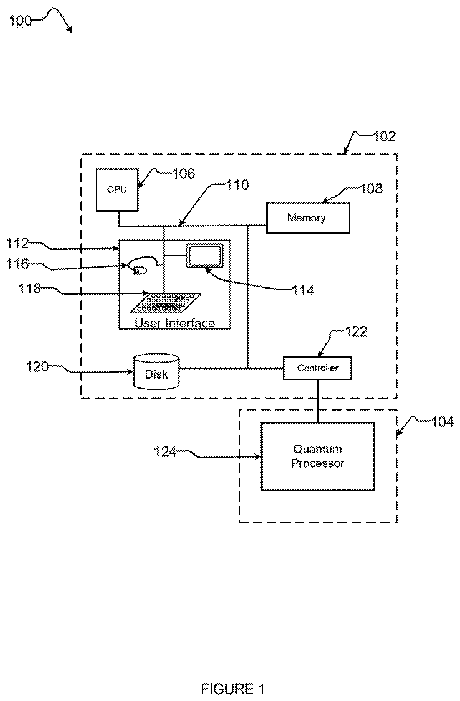
[0023] FIG. 1 is a schematic diagram of an example hybrid computing system comprising an analog processor and a digital processor.
[0024] FIG. 2 is a flow diagram showing an example method for calibrating devices in a quantum processor by determining optimized optimal parameter offset.
[0025] FIG. 3 is a flow diagram showing an example method to estimate flux noise in a quantum processor.
[0026] FIG. 4 is a flow diagram showing an example method for parameterizing the local iterative flux estimator in a quantum processor.
DETAILED DESCRIPTION
[0027] In the following description, certain specific details are set forth in order to provide a thorough understanding of various disclosed implementations. However, one skilled in the relevant art will recognize that implementations may be practiced without one or more of these specific details, or with other methods, components, materials, etc. In other instances, well-known structures associated with computer systems, server computers, and/or communications networks have not been shown or described in detail to avoid unnecessarily obscuring descriptions of the implementations.
[0028] Unless the context requires otherwise, throughout the specification and claims that follow, the word "comprising" is synonymous with "including," and is inclusive or open-ended (i.e., does not exclude additional, unrecited elements or method acts).
[0029] Reference throughout this specification to "one implementation" or "an implementation" means that a particular feature, structure or characteristic described in connection with the implementation is included in at least one implementation. Thus, the appearances of the phrases "in one implementation" or "in an implementation" in various places throughout this specification are not necessarily all referring to the same implementation. Furthermore, the particular features, structures, or characteristics may be combined in any suitable manner in one or more implementations.
[0030] As used in this specification and the appended claims, the singular forms "a," "an," and "the" include plural referents unless the context clearly dictates otherwise. It should also be noted that the term "or" is generally employed in its sense including "and/or" unless the context clearly dictates otherwise.
[0031] The headings and Abstract of the Disclosure provided herein are for convenience only and do not interpret the scope or meaning of the implementations.
[0032] FIG. 1 illustrates a hybrid computing system 100 including a digital computer 102 coupled to an analog computer 104. The example digital computer 102 is a classical computer 102 that includes a digital processor (CPU) 106 that may be used to perform classical digital processing tasks.
[0033] Classical computer 102 may include at least one digital processor (such as central processor unit 106 with one or more cores), at least one system memory 108, and at least one system bus 110 that couples various system components, including system memory 108 to central processor unit 106. The digital processor may be a logic processing unit, such as one or more central processing units ("CPUs"), graphics processing units ("GPUs"), digital signal processors ("DSPs"), application-specific integrated circuits ("ASICs"), programmable gate arrays ("FPGAs"), programmable logic controllers (PLCs), etc.
[0034] Classical computer 102 may include a user input/output subsystem 112. In some implementations, the user input/output subsystem includes one or more user input/output components such as a display 114, mouse 116, and/or keyboard 118.
[0035] System bus 110 can employ any known bus structures or architectures, including a memory bus with a memory controller, a peripheral bus, and a local bus. System memory 108 may include non-volatile memory, such as read-only memory ("ROM"), static random-access memory ("SRAM"), Flash NANO; and volatile memory such as random-access memory ("RAM") (not shown).
[0036] Classical computer 102 may also include other non-transitory computer or processor-readable storage media or non-volatile memory 120. Non-volatile memory 120 may take a variety of forms, including: a hard disk drive for reading from and writing to a hard disk, an optical disk drive for reading from and writing to removable optical disks, and/or a magnetic disk drive for reading from and writing to magnetic disks. The optical disk can be a CD-ROM or DVD, while the magnetic disk can be a magnetic floppy disk or diskette. Non-volatile memory 120 may communicate with the digital processor via system bus 110 and may include appropriate interfaces or controllers 122 coupled to system bus 110. Non-volatile memory 120 may serve as long-term storage for processor- or computer-readable instructions, data structures, or other data (sometimes called program modules) for classical computer 102.
[0037] Although classical computer 102 has been described as employing hard disks, optical disks and/or magnetic disks, those skilled in the relevant art will appreciate that other types of non-volatile computer-readable media may be employed, such magnetic cassettes, flash memory cards, Flash, ROMs, smart cards, etc. Those skilled in the relevant art will appreciate that some computer architectures employ volatile memory and non-volatile memory. For example, data in volatile memory can be cached to non-volatile memory, or a solid-state disk that employs integrated circuits to provide non-volatile memory.
[0038] Various processor- or computer-readable instructions, data structures, or other data can be stored in system memory 108. For example, system memory 108 may store instruction for communicating with remote clients and scheduling use of resources including resources on the classical computer 102 and analog computer 104. For example, the system memory 108 may store processor- or computer-readable instructions, data structures, or other data which, when executed by a processor or computer causes the processor(s) or computer(s) to execute one, more or all of the acts of the methods 200, 300 and 400 of FIGS. 2, 3, and 4, respectively.
[0039] In some implementations system memory 108 may store processor- or computer-readable instructions to perform pre-processing, co-processing, and post-processing by classical computer 102. System memory 108 may store at set of quantum computer interface instructions to interact with the analog computer 104.
[0040] Analog computer 104 may take the form of a quantum computer. Quantum computer 104 may include one or more quantum processors such as quantum processor 124. The quantum computer 104 can be provided in an isolated environment, for example, in an isolated environment that shields the internal elements of the quantum computer from heat, magnetic field, and other external noise (not shown). Quantum processor 124 includes programmable elements such as qubits, couplers and other devices. In accordance with the present disclosure, a quantum processor, such as quantum processor 124, may be designed to perform quantum annealing and/or adiabatic quantum computation. Example of quantum processor are described in U.S. Pat. No. 7,533,068.
[0041] The programmable elements of quantum processor 124, such as, for example, qubits, couplers, Digital to Analog Converters (DACs), readout elements, and other devices need to be calibrated. A calibration may be performed before quantum processor 124 is operated for the first time. Additionally, it may be advantageous to perform a calibration every time there is a change in the isolated environment of quantum processor 124, for example during a regular maintenance. Calibrating the devices of a quantum processor is advantageous to obtain well balanced samples from problems, including easy problems (e.g., independent spins) and hard problems (e.g., sampling, optimization of large, frustrated problems), to be solved with the quantum processor. The quantum processor may need to be programmed with a problem to be solved, for example by a digital or classical processor, before being operated.
[0042] Calibration methods for the devices or elements comprising quantum processors have been implemented with the aim of at least reducing unwanted time-dependent biases.
[0043] Elements in quantum processors are known to exhibit a respective noise spectrum that spans a wide range of frequencies, characterized by a 1/f spectrum. Therefore, samples used for statistical studies cannot be assumed to be independent, even on long time scales. Current calibration methods are only verified empirically, for example, by ad-hoc criteria, and, therefore, offer no theoretical guarantee for usefulness or correctness.
[0044] The present disclosure describes systems and methods to evaluate calibration procedures assuming only a given power spectral density and to determine parameter offsets to be used in a calibration procedure assuming only the power spectral density. The present methods may be executed by a hybrid computing system, for example hybrid computing system 100 of FIG. 1.
[0045] A statistically measurable scalar quantity m of a device of a quantum processor, associated with a known noise process .PHI. and calibration adjustment parameter .PHI..sup.0, can be described via a model P(m|.PHI., .PHI..sup.0). An example of scalar quantity m is the spin-state of a single qubit (or magnetization of a group of qubits), which spin-state or magnetization is linked to flux noise .PHI. and a flux offset parameter .PHI..sup.0. The form of the spectral density PSD (.PHI.) can be measured or computed, for example by assuming a combination of statistical error, 1/f spectrum and white noise.
[0046] The noise spectrum of the measurements can be approximated by a noise distribution over discrete frequencies, aligned with a discrete time measurement process on m. For regular data intervals, e.g., hourly calibration routines, successive reads or successive programming, the discretization of the noise spectrum can be robust. In some implementations, the discrete distribution may not be continuous, and may have missing values. These missing values may be inferred during the calibration process. The spectrum high frequency cut-off is either controlled by the read time for a single sample (e.g., 0 (.mu.s)), single programming (e.g., 0 (ms)), or between calibration updates, which can range from minutes to hours. The low frequency cut-off can represent the time-scale on which a device in the quantum processor should be calibrated, for example the duration of an experiment or the lifetime of the device.
[0047] In one implementation, the spectral density may be determined by running the analog processor and measuring the spectral density of the analog processor and sending this spectral density data to the digital computer. The power spectral density may also be determined at the same time as the flux biases or flux offsets are determined, using the Empirical Bayes Approach.
[0048] A probability distribution over the noise process (also referred in the present disclosure as sequence), for example the noise process of a qubit's flux, can be constructed based only on the spectrum. The probability distribution may be represented or expressed as an integral. The probability distribution can be used to choose a parameter calibration adjustment on the next programming of 0.degree. , to at least reduce errors. For example, spin states (or magnetization over a plurality of programming of the quantum processor) are expected to be zero biased (i.e., non-biased) in absence of programmed external biases. Therefore, it is desirable to choose a flux offset of a qubit on the next programming in order to minimize the expected distance between the average spin value and the known value (i.e., 0).
[0049] The integral representing the probability distribution can be evaluated, for example by Monte-Carlo or Markov Chain Monte Carlo (MCMC) methods, to determine the optimal parameter setting, therefore achieving optimal performance under well-defined theoretical assumptions that account for time dependence. In the present disclosure and appended claims, optimal parameter settings (or optimized parameter settings) are parameter settings that reduce time dependent biases in the elements of a quantum processor. Other techniques, such as approximate sampling, heuristic optimization, or optimization using a quantum processing unit (QPU) may also be used.
[0050] For simplicity, the following description will refer to calibrating the flux of a qubit in a quantum processor, and measurements of magnetization for independent spins, for example one magnetization measurement per programming of the quantum processor, with roughly evenly spaced programmings (e.g., once per hour). However, other statistics pertinent to the calibration of a quantum processor can be considered. In addition, the samples, or measurements, may not be evenly spaced.
[0051] For notational convenience, and assuming time reversal symmetry of the noise process, the systems and methods in the present disclosure will be described presuming the time running backwards. For example, systems and methods are described to predict the flux noise at time 0, given known values for the flux offset .PHI..sup.0 and magnetizations m for t.di-elect cons.[1, T.sub.D], where T.sub.D is the number of discrete data points, alongside a longer background noise process, extending to T>>T.sub.D (e.g., a factor 10).
[0052] The relationship between the data (m) flux process noise, the sampling flux offset and the measured magnetization m.sub.t at time t is given by the thermal relation under the freeze-out hypothesis (discussed, for example, in Amin (https://arxiv.org/pdf/1503.04216.pdf%E2%80%8B)), which is well established for independent spins:
m.sub.t=f(.PHI..sub.t.sup.0, .PHI..sub.t)=tan h(.beta.*[.PHI..sub.t.sup.0+.PHI..sub.t])+n.sub.t (1)
[0053] Where n.sub.t is the random sampling error of measuring m well approximated by a Gaussian distribution N(0, 1/n.sub.s) independent of .PHI., .PHI..sup.0 and t if enough independent samples n.sub.s are drawn or measured and .PHI..sub.t.sup.0.apprxeq..PHI..sub.t, and .beta. is a freeze-out inverse temperature parameter.
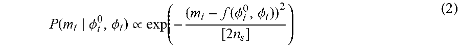
[0054] Thus, the likelihood of the data given the sequences is defined as:
P ( m t .phi. t 0 , .phi. t ) .varies. exp ( - ( m t - f ( .phi. t 0 , .phi. t ) ) 2 [ 2 n s ] ) ( 2 ) ##EQU00001##
[0055] In the case of .PHI..sub.t.sup.0.apprxeq..PHI..sub.t, f can be linearized, and the sampling noise n.sub.t is equivalent to additional white noise on the flux.
[0056] The systems and methods herein described can be specified by approximating the dependence of m on flux parameters [.PHI..sub.t.sup.0+.PHI..sub.t] as linear, this being generally applicable in the limit of nearly calibrated regime where errors are small. Therefore, the present systems and methods can be applied to calibration of systems of strongly coupled variables, and are not limited to single-spin of a qubit or single-chain of qubits. Calibrating one qubit, or one logical qubit (i.e., a plurality of qubits coupled or chained together so as to behave like a single qubit), at a time for large coupled problems may be inefficient for situations where spins are coupled and something about the coupling is known. For example, if the pattern of correlations is known, patterns in the impact of the control parameters (directions of high susceptibility) can be identified, and these directions (where signal to noise ratio is higher) can be calibrated more accurately.
[0057] Relation between the discrete noise spectrum and the discretized real time noise process is given by the inverse Fourier Transform.
.phi. t = .omega. = T / 2 T / 2 - 1 .phi. .omega. exp ( i 2 .pi. .omega. t / T ) ( 3 ) ##EQU00002##
[0058] where .PHI..sub.t is the signal in the time space, .PHI..sub..omega. is the signal in frequency space and T is the length of sequence to be transformed. Eq. (3) defines a deterministic relationship P({.PHI..sub.t}|{.PHI..sub..omega.}), but both variables .PHI..sub.t and .PHI..sub..omega. can be treated as random variables for simplicity. One variable type or the other, for example .PHI..sub.t, will be explicitly integrated out once the distribution of interest is determined.
[0059] The power distribution in frequency space .PHI..sub..omega. is known, therefore, no assumptions are necessary to define a probability distribution over the frequency fluxes from the power spectral density for the non-negative frequency components
P ( { .phi. .omega. } ) .varies. .omega. exp ( - .phi. .omega. 2 / [ 2 P S D ( .omega. ) ] ( 4 ) ##EQU00003##
[0060] Where the negative components are conjugate (since the noise sequence is real):
.PHI..sub..omega.=.PHI.*.sub.-.omega..
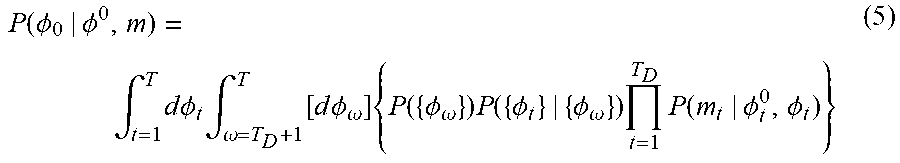
[0061] Under the above assumptions, the probability distribution of the data for the next data point, or flux noise on the next data point can be represented or expressed as:
P ( .phi. 0 | .phi. 0 , m ) = .intg. t = 1 T d .phi. t .intg. .omega. = T D + 1 T [ d .phi. .omega. ] { P ( { .phi. .omega. } ) P ( { .phi. t } | { .phi. .omega. } ) t = 1 T D P ( m t | .phi. t 0 , .phi. t ) } ( 5 ) ##EQU00004##
[0062] where .PHI..sub.0 is the value of .PHI..sub.t at time t=0 (the next value in the noise sequence). It is possible to integrate out either {.PHI..sub.t} or {.PHI..sub..omega.}. Depending on the spectral properties it may be advantageous to integrate out one or the other variable. An example where integration of .PHI..sub.t is favorable is when only a narrow range (or sparse subset) of frequencies require modelling. In the example of 1/f noise, only the lower frequency must be modeled with high accuracy, approximating the higher frequency elements by white noise--in this case integrating out the large number of time variables leaves only a relatively small problem to solve. By contrast, if there are relative few unknown time components (e.g., T.about.T.sub.D, with no data gaps) it becomes advantageous to integrate out the frequencies, leaving only the relatively small number of unknown time elements.
[0063] In addition, it is also possible to make the integral of significantly lower dimension by explicitly modelling all of the high frequency components as white noise, thus, leaving a very sparse representation for PSD(.PHI.) over only the lowest frequencies.
[0064] Eq. (5) can be evaluated via Monte Carlo or Markov Chain Monte Carlo methods. However, other methods for evaluating the integral can employed, for example, maximizing the probability of the unknown parameters (i.e., working with the most likely flux sequences, instead of a distribution over flux sequences, or maximum likelihood estimators).
[0065] The systems and methods of the present disclosures can be used, for example, to estimate the ideal flux offset of a qubit. Determining correctly the flux offset will lead to reduced error on any measurements sensitive to noise on the next step, given a history of calibrations. An appropriate flux offset setting will bring magnetization close to zero, by appropriate choice of .PHI..sub.0.sup.0. Since the noise distribution is expected to be Gaussian-like and the error is expected to be roughly symmetric, setting .PHI..sub.0.sup.0=-argmax.sub..PHI..sub.0P(.PHI..sub.0|.PHI..sup.0, m) will estimate an ideal flux offset. The flux offset can be estimated by integration or by approximation to the integral (e.g., maximizing with respect to the integration parameters).
[0066] Algorithm 1 (see below) contains pseudocode for estimating the ideal flux offset of a qubit.
TABLE-US-00001 Algorithm 1 // MAP estimator : Inputs : f ( ) , T , n_S {phi{circumflex over ( )}0_t , m_t : t=1 , . . , T_D } , PSD Output : \phi_0 : Estimate of the flux noise on the next step \\ (set \ phi{circumflex over ( )}0_0 = - \ phi_0 to compensate ) Method : gradient descent of P(\ phi_0 | \phi{circumflex over ( )}0,m)) in {\phi_\omega } or integrate P(\phi_0 | \phi{circumflex over ( )}0,m)) by MCMC: \\ fit \phi_0 distribution by a Gaussian and take maxima.
[0067] The systems and methods described in the present disclosure can be used, for example, for parameterizing local iterative flux estimators. The error for choosing the next flux offset .PHI..sub.0.sup.0 can be calculated according to some a parameterized rule R.sub..alpha.(.PHI..sup.0, m), where .alpha. represents an optimal parameter for successive iteration of calibration. An example of an iterative rule to minimize the variance of magnetization is R.sub..alpha.(.PHI..sup.0, m): .PHI..sub.t+1=.PHI..sub.t+.alpha.m.sub.t. For example, the mean square error can be minimized as follows:
.alpha.=argmin.sub..alpha.Error(.alpha.)-argmin.sub..alpha..intg.d.PHI..- sub.0P(.PHI..sub.0|.PHI..sup.0, m)f(R.sub..alpha.(.PHI..sup.0, m), .PHI..sub.0).sup.2 (6)
[0068] Using EQ (6) may be advantageous given that a needs to be determined only once. Also, EQ (6) may be more robust to imperfections (e.g., unmodelled effects like occasional readout errors) whilst correctly identifying trends related to bulk noise properties (e.g., how to adjust .alpha. in the case of lower mid-band noise).
[0069] Since parameterizing the estimator is a one-time effort, it may be worth explicitly integrating EQ (6) via MCMC to high precision to obtain a more accurate result. Alternatively, maximizing the integration variables to evaluate EQ (6) is also possible. Algorithm 2 (see below) contains pseudocode for optimizing calibration parameters.
TABLE-US-00002 Algorithm 2 // Optimizing parameters of robust shim methods : Inputs : f( ) , R( ) , T, n_S {phi{circumflex over ( )}0_t , m_t : t=1 ,.., T_D }, \alpha Output : \alpha : Optimal parameter for iterative shimming method \\ Method: Solve equation (6) by integration, \\ Or optimization , of unknown noise process parameters.
[0070] The systems and methods described in the present disclosure can be used, for example, for determining a probability for the full unseen noise process P(.PHI.|.PHI..sup.0, m), thus allowing extrapolation or interpolation. The distribution over any flux can be determined historically, or a subsequent distribution can be determined by marginalization or by directly sampling full sequences from the determined distribution. The probability distribution can be used to conduct statistically significant testing, or importance sampling, of historical data to better improve estimators or properly evaluate the uncertainty of the experiment, for example, by bootstrapping methods. As used herein, calibration parameter a may be a single value, a set of values, or a function of time.
[0071] FIG. 2 shows an example method 200 for calibrating devices in a quantum processor by determining optimal parameter offset. Method 200 may be executed on a hybrid computing system comprising an analog processor and a digital processor, for example hybrid computing system 100 having a classical and a quantum processor of FIG. 1.
[0072] Method 200 comprises acts 201 to 207; however, a person skilled in the art will understand that the number of acts is an example and, in some implementations, certain acts may be omitted, further acts may be added, and/or the order of the acts may be changed.
[0073] Method 200 starts at 201, for example in response to a call from another routine.
[0074] At 202, hybrid computing system 100 receives a model. The digital processor may determine a model P(m.sub.t|.PHI..sub.t.sup.0, .PHI..sub.t) for a measurable quantity m associated with a noise process .PHI. and an offset parameter .PHI..sup.0. An example model is given in EQ (2). Alternatively, hybrid computing system receives the model as part of a set of inputs and includes the appropriate parameter values. In one implementation, the model may be a theoretical model that is provided as an input.
[0075] At 203, hybrid computing system 100 receives a spectral density PSD(.PHI.). Hybrid computing system 100 may measure m to determine PSD(.PHI.) or hybrid computing system 100 may computed the form of PSD(.PHI.), for example assuming a combination of statistical error, 1/f spectrum and white noise. In one implementation, the spectral density may be a theoretical spectral density that is provided as an input.
[0076] At 204, hybrid computing system 100 approximates a noise spectrum by a discrete distribution, aligned with a discrete measurement process on m. Hybrid computing system 100 determines a relationship P({.PHI..sub.t}, {.PHI..sub..omega.}) between the signal in the time space .PHI..sub.t and the signal in the frequency space .PHI..sub..omega.. The relation between the discrete noise process and the discretized real time noise process is given by the inverse Fourier transform of EQ (3). As noted above, the discrete distribution may not have continuous intervals, and missing values may be inferred.
[0077] At 205, hybrid computing system 100 constructs a probability distribution of the noise process based on the discrete distribution, as described above with reference to EQ (5). Hybrid computing system 100 uses the deterministic relationship P({.PHI..sub.t}, {.PHI..sub..omega.}) determined at 204, and the model determined at 202 to arrive at the probability distribution of EQ (5). In one implementation, the probability distribution may be a probability distribution of the noise process over time. In another implementation, the probability distribution may be a probability distribution of the noise process over a frequency space.
[0078] At 206, hybrid computing system 100 evaluates the probability distribution constructed at 205. The probability distribution may be evaluated by Monte Carlo or Markov Chain Monte Carlo methods. The probability distribution may also be evaluated by approximate sampling, a heuristic optimization method, or optimization by the analog processor.
[0079] At 207, method 200 terminates, until it is, for example, invoked again.
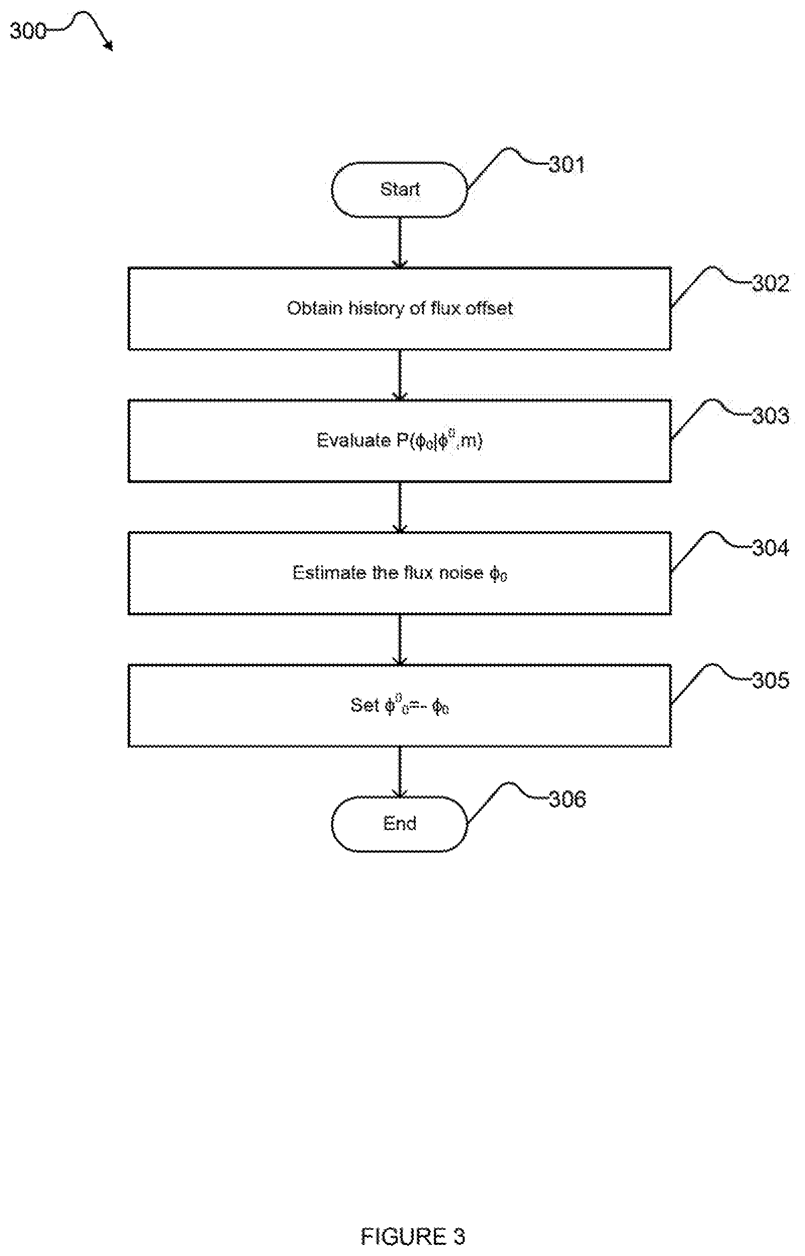
[0080] FIG. 3 shows an example method 300 to estimate flux noise in a quantum processor. Method 300 may be executed on a hybrid computing system comprising a classical and a quantum processor, for example hybrid computing system 100 of FIG. 1.
[0081] Method 300 comprises acts 301 to 306; however, a person skilled in the art will understand that the number of acts is an example and, in some implementations, certain acts may be omitted, further acts may be added, and/or the order of the acts may be changed.
[0082] Method 300 starts at 301, for example in response to a call from another routine.
[0083] At 302, hybrid computing system 100 obtains a history of a noise in a parameter measurement. In one implementation, hybrid computing 100 obtains a history of a flux noise of a qubit. For example, hybrid computing system 100 may obtain independent samples n.sub.s{.PHI..sub.t.sup.0, m.sub.t: t=1, . . . T.sub.D}, f(.PHI..sub.t.sup.0, .PHI..sub.t), a spectral density PSD(.PHI.), and a probability distribution P(.PHI..sub.0|.PHI..sup.0, m), as described in method 200 of FIG. 2.
[0084] At 303, hybrid computing system 100 evaluates the probability distribution P(.PHI..sub.0|.PHI..sup.0, m) from EQ (5). In one implementation, P(.PHI..sub.0|.PHI..sup.0, m) is evaluated by gradient descent in {.PHI..sub..omega.}. Alternatively, P(.PHI..sub.0|.PHI..sup.0, m) is evaluated by integration via Markov Chain Monte Carlo.
[0085] At 304, hybrid computing system 100 estimates .PHI..sub.0 (e.g., the flux noise on the next calibration). In one implementation, the .PHI..sub.0 distribution is fitted to a Gaussian distribution and the maxima taken.
[0086] At 305, hybrid computing system 100 sets the next flux offset .PHI..sub.0.sup.0=-.PHI..sub.0 to compensate the flux noise.
[0087] At 306, method 300 terminates, until it is, for example, invoked again.
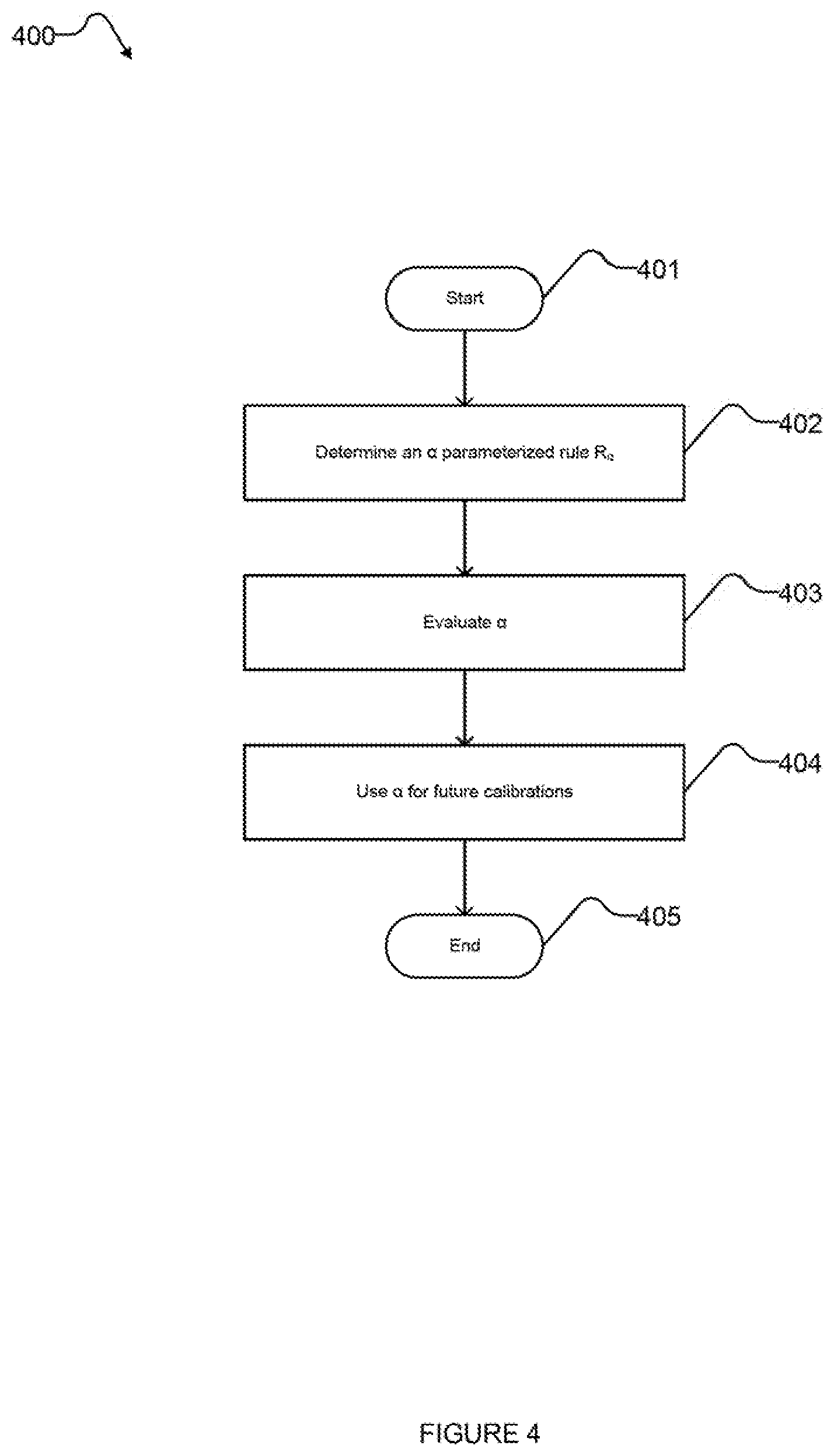
[0088] FIG. 4 shows an example method 400 for parameterizing a local iterative flux estimator in a quantum processor. Method 400 may be executed on a hybrid computing system comprising a classical and a quantum processor, for example hybrid computing system 100 of FIG. 1.
[0089] Method 400 comprises acts 401 to 405; however, a person skilled in the art will understand that the number of acts is an example and, in some implementations, certain acts may be omitted, further acts may be added, and/or the order of the acts may be changed.
[0090] Method 400 starts at 401, for example in response to a call from another routine.
[0091] At 402, hybrid computing system 100 determines an .alpha. parameterized rule R.sub..alpha.(.PHI..sup.0, m) to choose the next flux offset .PHI..sub.0.sup.0, where .alpha. is defined as an optimal parameter to be used for future calibrations. In at least one implementation R.sub..alpha.(.PHI..sup.0, m): .PHI..sub.t+1=.PHI..sub.t+.alpha.m.
[0092] At 403, hybrid computing system 100 evaluates .alpha., where .alpha. is defined in EQ (6). In at least one implementation, EQ (6) is solved by integration, for example via MCMC. Alternatively, the variables in EQ (6) may be maximized to evaluate .alpha..
[0093] At 404, hybrid computing system 100 uses .alpha. as a calibration adjustment parameter for future calibrations of quantum computer 102.
[0094] At 405, method 400 terminates, until it is, for example, invoked again.
[0095] The above described method(s), process(es), or technique(s) could be implemented by a series of processor readable instructions stored on one or more nontransitory processor-readable media. Some examples of the above described method(s), process(es), or technique(s) method are performed in part by a specialized device such as an adiabatic quantum computer or a quantum annealer or a system to program or otherwise control operation of an adiabatic quantum computer or a quantum annealer, for instance a computer that includes at least one digital processor. The above described method(s), process(es), or technique(s) may include various acts, though those of skill in the art will appreciate that in alternative examples certain acts may be omitted and/or additional acts may be added. Those of skill in the art will appreciate that the illustrated order of the acts is shown for exemplary purposes only and may change in alternative examples. Some of the exemplary acts or operations of the above described method(s), process(es), or technique(s) are performed iteratively. Some acts of the above described method(s), process(es), or technique(s) can be performed during each iteration, after a plurality of iterations, or at the end of all the iterations.
[0096] The above description of illustrated implementations, including what is described in the Abstract, is not intended to be exhaustive or to limit the implementations to the precise forms disclosed. Although specific implementations of and examples are described herein for illustrative purposes, various equivalent modifications can be made without departing from the spirit and scope of the disclosure, as will be recognized by those skilled in the relevant art. The teachings provided herein of the various implementations can be applied to other methods of quantum computation, not necessarily the exemplary methods for quantum computation generally described above.
[0097] The various implementations described above can be combined to provide further implementations. All of the commonly assigned US patent application publications, US patent applications, foreign patents, and foreign patent applications referred to in this specification and/or listed in the Application Data Sheet are incorporated herein by reference, in their entirety, including but not limited to: U.S. Provisional Patent Application No. 62/855,512 and U.S. Pat. No. 7,533,068.
[0098] These and other changes can be made to the implementations in light of the above-detailed description. In general, in the following claims, the terms used should not be construed to limit the claims to the specific implementations disclosed in the specification and the claims, but should be construed to include all possible implementations along with the full scope of equivalents to which such claims are entitled. Accordingly, the claims are not limited by the disclosure.
* * * * *
References
D00000
D00001
D00002
D00003
D00004
XML
uspto.report is an independent third-party trademark research tool that is not affiliated, endorsed, or sponsored by the United States Patent and Trademark Office (USPTO) or any other governmental organization. The information provided by uspto.report is based on publicly available data at the time of writing and is intended for informational purposes only.
While we strive to provide accurate and up-to-date information, we do not guarantee the accuracy, completeness, reliability, or suitability of the information displayed on this site. The use of this site is at your own risk. Any reliance you place on such information is therefore strictly at your own risk.
All official trademark data, including owner information, should be verified by visiting the official USPTO website at www.uspto.gov. This site is not intended to replace professional legal advice and should not be used as a substitute for consulting with a legal professional who is knowledgeable about trademark law.