Analog-circuit Fault Diagnosis Method Based On Continuous Wavelet Analysis And Elm Network
HE; Yigang ; et al.
U.S. patent application number 16/088079 was filed with the patent office on 2020-09-24 for analog-circuit fault diagnosis method based on continuous wavelet analysis and elm network. This patent application is currently assigned to HEFEI UNIVERSITY OF TECHNOLOGY. The applicant listed for this patent is HEFEI UNIVERSITY OF TECHNOLOGY. Invention is credited to Liulu HE, Wei HE, Yigang HE, Zhigang LI, Qiwu LUO, Luqiang SHI, Tiancheng SHI, Tao WANG, Zhijie YUAN, Deqin ZHAO.
| Application Number | 20200300907 16/088079 |
| Document ID | / |
| Family ID | 1000004887200 |
| Filed Date | 2020-09-24 |


View All Diagrams
| United States Patent Application | 20200300907 |
| Kind Code | A1 |
| HE; Yigang ; et al. | September 24, 2020 |
ANALOG-CIRCUIT FAULT DIAGNOSIS METHOD BASED ON CONTINUOUS WAVELET ANALYSIS AND ELM NETWORK
Abstract
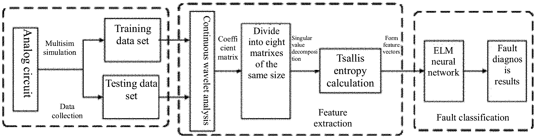
An analog-circuit fault diagnosis method based on continuous wavelet analysis and an ELM network comprises: data acquisition: performing data sampling on output responses of an analog circuit respectively through Multisim simulation to obtain an output response data set; feature extraction: performing continuous wavelet analysis by taking the output response data set of the circuit as training and testing data sets respectively to obtain a wavelet time-frequency coefficient matrix, dividing the coefficient matrix into eight sub-matrixes of the same size, and performing singular value decomposition on the sub-matrixes to calculate a Tsallis entropy for each sub-matrix to form feature vectors of corresponding faults; and fault classification: submitting the feature vector of each sample to the ELM network to implement accurate and quick fault classification. The method of the invention has a better effect on extracting the circuit fault features and can be used to implement circuit fault classification accurately and efficiently.
| Inventors: | HE; Yigang; (Anhui, CN) ; HE; Wei; (Anhui, CN) ; LUO; Qiwu; (Anhui, CN) ; LI; Zhigang; (Anhui, CN) ; SHI; Tiancheng; (Anhui, CN) ; WANG; Tao; (Anhui, CN) ; YUAN; Zhijie; (Anhui, CN) ; ZHAO; Deqin; (Anhui, CN) ; SHI; Luqiang; (Anhui, CN) ; HE; Liulu; (Anhui, CN) | ||||||||||
| Applicant: |
|
||||||||||
|---|---|---|---|---|---|---|---|---|---|---|---|
| Assignee: | HEFEI UNIVERSITY OF
TECHNOLOGY Anhui CN |
||||||||||
| Family ID: | 1000004887200 | ||||||||||
| Appl. No.: | 16/088079 | ||||||||||
| Filed: | January 6, 2017 | ||||||||||
| PCT Filed: | January 6, 2017 | ||||||||||
| PCT NO: | PCT/CN2017/070351 | ||||||||||
| 371 Date: | September 25, 2018 |
| Current U.S. Class: | 1/1 |
| Current CPC Class: | G01R 31/316 20130101; G01R 31/2846 20130101 |
| International Class: | G01R 31/28 20060101 G01R031/28; G01R 31/316 20060101 G01R031/316 |
Foreign Application Data
| Date | Code | Application Number |
|---|---|---|
| Dec 29, 2016 | CN | 201611243708.5 |
Claims
1. An analog-circuit fault diagnosis method based on a continuous wavelet analysis and an ELM neural network, comprising three steps of data acquisition, feature extraction and fault classification, wherein the step of data acquisition comprises: performing a data sampling on an output end of an analog circuit to obtain an output response data set, wherein the step of feature extraction comprises: performing a continuous wavelet transform by taking the output response data set as a training data set and a testing data set respectively to obtain a wavelet time-frequency coefficient matrix of fault signals; dividing the wavelet time-frequency coefficient matrix into eight sub-matrixes of the same size; performing a singular value decomposition on the sub-matrixes to obtain a plurality of singular values; and calculating a Tsallis entropy value for the singular values of each sub-matrix, wherein the Tsallis entropy values form corresponding circuit response fault feature vectors, and wherein the step of fault classification comprises: inputting the circuit response fault feature vectors into the ELM neural network to implement a fault classification for the analog circuit.
2. The analog-circuit fault diagnosis method based on the continuous wavelet analysis and the ELM neural network according to claim 1, wherein the wavelet time-frequency coefficient matrix is obtained from the following formula: W.sub.x(.tau.,a)= {square root over (a)}.intg..sub.-.infin..sup.+.infin.x(t).phi.(a(t-.tau.))dt=<x,.phi..s- ub..tau.,a> (1), wherein W.sub.x(.tau.,a) represents a continuous wavelet transform time-frequency coefficient matrix of a signal x(t), .tau. and a represent a time parameter and a frequency parameter for the continuous wavelet transform respectively, with a>0, .phi.(t) represents a wavelet generating function, and .phi..sub..tau.,a(t) represents a wavelet basis function which is a set of function series formed by dilation and translation of the wavelet generating function .phi.(t) and satisfies the following formula: .PHI. .tau. , a ( t ) = 1 a .PHI. ( t - .tau. a ) . ( 2 ) ##EQU00011##
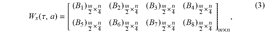
3. The analog-circuit fault diagnosis method based on the continuous wavelet analysis and the ELM neural network according to claim 1, wherein the eight sub-matrixes obtained by dividing the wavelet time-frequency coefficient matrix are represented by the following formula: W x ( .tau. , a ) = [ ( B 1 ) m 2 .times. n 4 ( B 2 ) m 2 .times. n 4 ( B 3 ) m 2 .times. n 4 ( B 4 ) m 2 .times. n 4 ( B 5 ) m 2 .times. n 4 ( B 6 ) m 2 .times. n 4 ( B 7 ) m 2 .times. n 4 ( B 8 ) m 2 .times. n 4 ] m .times. n , ( 3 ) ##EQU00012## wherein W.sub.x(.tau.,a) represents a m.times.n-dimension wavelet time-frequency coefficient matrix, and B.sub.1,B.sub.2,B.sub.3,B.sub.4,B.sub.5,B.sub.6,B.sub.7,B.sub.8 represent the eight sub-matrixes obtained through division.
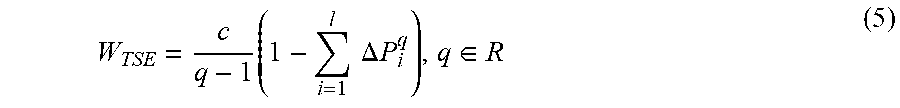
4. The analog-circuit fault diagnosis method based on the continuous wavelet analysis and the ELM neural network according to claim 1, wherein the singular values obtained by performing the singular value decomposition on the sub-matrixes are represented by the following formula: B.sub.c.times.d=U.sub.c.times.lA.sub.l.times.lV.sub.l.times.d (4), wherein B.sub.c.times.d represents the c.times.d-dimension sub-matrixes obtained after the division via the formula (3); and a plurality of principal diagonal elements .lamda..sub.i(i=1, 2, . . . , l) of A are the singular values of B.sub.c.times.d with .lamda..sub.1.gtoreq..lamda..sub.2.gtoreq. . . . .gtoreq..lamda..sub.l.gtoreq.0, wherein l is the number of non-zero singular values, wherein the step of calculating the Tsallis entropy value for the singular values of each sub-matrix is represented by the following formula: W TSE = c q - 1 ( 1 - i = 1 l .DELTA. P i q ) , q .di-elect cons. R , ( 5 ) ##EQU00013## wherein W.sub.TSE represents the Tsallis entropy value as calculated, .DELTA. P i = - ( .lamda. i j = 1 l .lamda. j ) log ( .lamda. i j = 1 l .lamda. j ) , ##EQU00014## and q represents a non-extensive parameter, with c=1 and q=1.2, wherein the Tsallis entropy values of the singular values of respective sub-matrixes as calculated with the formula (5) are combined together to form the corresponding circuit response fault feature vectors.
5. The analog-circuit fault diagnosis method based on the continuous wavelet analysis and the ELM neural network according to claim 2, wherein the eight sub-matrixes obtained by dividing the wavelet time-frequency coefficient matrix are represented by the following formula: W x ( .tau. , a ) = [ ( B 1 ) m 2 .times. n 4 ( B 2 ) m 2 .times. n 4 ( B 3 ) m 2 .times. n 4 ( B 4 ) m 2 .times. n 4 ( B 5 ) m 2 .times. n 4 ( B 6 ) m 2 .times. n 4 ( B 7 ) m 2 .times. n 4 ( B 8 ) m 2 .times. n 4 ] m .times. n , ( 3 ) ##EQU00015## wherein W.sub.x(.tau.,a) represents a m.times.n-dimension wavelet time-frequency coefficient matrix, and B.sub.1,B.sub.2,B.sub.3,B.sub.4,B.sub.5,B.sub.6,B.sub.7,B.sub.8 represent the eight sub-matrixes obtained through division.
Description
FIELD OF THE INVENTION
[0001] The invention relates to an analog-circuit fault diagnosis method, and in particular to an analog-circuit fault diagnosis method based on a continuous wavelet analysis and an ELM network.
DESCRIPTION OF RELATED ART
[0002] Analog circuits play an extremely important role in fields such as consumer electronics, industry, aerospace and military. Once an analog circuit fails, the performance and function of an electronic device would be affected, resulting in slow response, functional failure or even catastrophic consequences of the device. Meanwhile, with the increasing complexity and intensity of electronic devices, the analog circuit is characterized by nonlinearity, device tolerance and response continuity. As such, there are great challenges existing in the fault location and elimination for the analog circuits, and how to design an analog-circuit fault diagnosis method with high accuracy and strong instantaneity has become a current and difficult subject in this field.
[0003] Regarding the fault diagnosis of the analog circuits, many scholars have adopted the wavelet analysis and neural network respectively as the core technologies for the fault feature extraction and fault classification. Relevant references are as follows: "Spina R, Upadhyaya S. Linear circuit fault diagnosis using neuromorphic analyzers [J]. Circuits & Systems II Analog & Digital Signal Processing IEEE Transactions on, 1997, 44(3):188-196." and "Negnevitsky M, Pavlovsky V. Neural Networks Approach to Online Identification of Multiple Failure of Protection Systems [J]. IEEE Transactions on Power Delivery, 2005, 20(2):588-594.", wherein unprocessed circuit output response signals are directly used as inputs for the neural network, however resulting in overlong training time for the neural network and overlow diagnosis accuracy; "Aminian M, Aminian F. Neural-network based analog-circuit fault diagnosis using wavelet transform as preprocessor [J]. IEEE Transactions on Circuits & Systems II Analog & Digital Signal Processing, 2000, 47(2):151-156.", wherein low-frequency wavelet coefficients subjected to principal component analysis treatment are submitted to the neural network as fault features, which increases the accuracy of fault diagnosis but makes no substantial improvement to the complexity of the network; and "He Xing, Wang Hongli, Lu Jinghui et. al. Analog Circuit Fault Diagnosis Method Based on Preferred Wavelet Packet and ELM[J]. Chinese Journal of Scientific Instruments, 2013, 34(11):2614-2619.", wherein the normalized energy values of respective node coefficients are analyzed by calculating wavelet packets and then taken as the fault features to reduce the complexity of the neural network, however, the energy values are very small to lead to insignificant feature distinction. Furthermore, in combination with the methods above, there are the following problems present in the prior art.
[0004] 1. When extracting the circuit fault features, the above methods usually discard detail wavelet coefficients but select the normalized energy values approximate to the wavelet coefficients as the fault features. From the perspective of information integrity, the discarded detail coefficients have a considerable value for the extracted features to fully reflect the fault information.
[0005] 2. The traditional feed forward neural network (such as BP, RBF) is a common classifier in the field of fault diagnosis, but there are problems such as slow network learning, susceptibility to locally optimal solution and over training.
SUMMARY OF THE INVENTION
[0006] In view of the above problems existing in the prior art, the technical problems to be solved by the invention are how to obtain the useful information of the fault response more completely; how to effectively describe the fault features so that the features are clearly distinguished from each other; and how to implement the fault classification more quickly and accurately, and an analog-circuit fault diagnosis method with continuous wavelet analysis and ELM network for fault feature extraction and fault classification respectively is thus provided.
The technical solution adopted by the invention to solve the technical problems thereof is as follows:
[0007] an analog-circuit fault diagnosis method based on a continuous wavelet transform and an ELM network comprises the following steps:
[0008] (1) data acquisition: performing a data sampling on an output end of an analog circuit to obtain an output response data set;
[0009] (2) feature extraction: performing a continuous wavelet transform by taking the output response data set as a training data set and a testing data set respectively to obtain a wavelet time-frequency coefficient matrix of fault signals, dividing the wavelet time-frequency coefficient matrix into eight sub-matrixes of the same size, performing a singular value decomposition on the sub-matrixes to obtain singular values, and calculating a Tsallis entropy for the singular values of each sub-matrix, wherein the Tsallis entropy values form corresponding circuit response fault feature vectors; and
[0010] (3) fault classification: inputting the circuit response fault feature vectors into an ELM neural network to implement the accurate and quick fault classification for the analog circuit.
[0011] Further, the data sampling in Step (1) is implemented through a Multisim simulation. The output response data set is time-domain output voltage signals of the analog circuit.
[0012] Further, the wavelet time-frequency coefficient matrix can be obtained through the following formula:
W.sub.x(.tau.,a)= {square root over (a)}.intg..sub.-.infin..sup.+.infin.x(t).phi.(a(t-.tau.))dt=<x,.phi..s- ub..tau.,a> (1),
[0013] here, W.sub.x(.tau., a) represents a continuous wavelet transform time-frequency coefficient matrix of a signal x(t); .tau. and a represent a time parameter and a frequency parameter for the continuous wavelet transform respectively, with a>0; .phi.(t) represents a wavelet generating function; .phi..sub..tau.,a(t) represents a wavelet basis function which is a set of function series formed by dilation and translation of the wavelet generating function .phi.(t), that is,
.PHI. .tau. , a ( t ) = 1 a .PHI. ( t - .tau. a ) . ( 2 ) ##EQU00001##
[0014] The eight sub-matrixes obtained by dividing the wavelet time-frequency coefficient matrix can be represented by the following formula:
W x ( .tau. , a ) = [ ( B 1 ) m 2 .times. n 4 ( B 2 ) m 2 .times. n 4 ( B 3 ) m 2 .times. n 4 ( B 4 ) m 2 .times. n 4 ( B 5 ) m 2 .times. n 4 ( B 6 ) m 2 .times. n 4 ( B 7 ) m 2 .times. n 4 ( B 8 ) m 2 .times. n 4 ] m .times. n , ( 3 ) ##EQU00002##
[0015] here, W.sub.x(.tau., a) represents a m.times.n-dimension wavelet time-frequency coefficient matrix, and B.sub.1,B.sub.2,B.sub.3,B.sub.4,B.sub.5,B.sub.6,B.sub.7,B.sub.8 here represent the eight sub-matrixes obtained through division.
[0016] The singular values obtained by performing the singular value decomposition on the sub-matrixes can be represented by the following formula:
B.sub.c.times.d=U.sub.c.times.lA.sub.l.times.lV.sub.l.times.d (4),
[0017] here, B.sub.c.times.d represents the c.times.d-dimension sub-matrixes obtained after the division via the formula (3); and principal diagonal elements .lamda..sub.i(i=1, 2, . . . , l) of A are the singular values of B.sub.a.times.b with .lamda..sub.1.gtoreq..lamda..sub.2.gtoreq. . . . .gtoreq..lamda..sub.l.gtoreq.0, wherein l is the number of non-zero singular values.
[0018] The step of calculating the Tsallis entropy for the singular value of each sub-matrix can be represented by the following formula:
W TSE = c q - 1 ( 1 - i = 1 l .DELTA. P i q ) , q .di-elect cons. R ( 5 ) ##EQU00003##
[0019] here, W.sub.TSE represents the Tsallis entropy value as calculated,
.DELTA. P i = - ( .lamda. i j = 1 l .lamda. j ) log ( .lamda. i j = 1 l .lamda. j ) , ##EQU00004##
and q represents a non-extensive parameter, with c=1 and q=1.2 in the invention.
[0020] The Tsallis entropy values of the singular values of respective sub-matrixes as calculated with the formula (5) are combined together to form corresponding circuit response fault feature vectors.
[0021] The extreme learning machine (ELM) is based on single-hidden layer feed forward networks (SLFNs), where an input weight and a hidden layer deviation are randomly assigned by setting an appropriate number for hidden layer nodes, and then a minimum norm least square solution obtained is directly used as a network output weight. Compared with the traditional feed forward neural network, ELM has strong learning ability and high processing speed, and meanwhile has the advantages of fewer parameters to be determined and high efficiency.
[0022] Compared with the prior art, the invention has the following advantages:
[0023] with the continuous wavelet transform, the invention acquires useful features of fault signals relatively completely, obtains eight sub-matrixes with completely the same size by a division method, highlights local minor changes of the matrixes, and further map fault information to an entropy space by calculating the Tsallis entropies of singular values of the respective sub-matrixes, thereby more finely describing the fault features (with extremely significant distinction among respective fault features and between the fault features and normal features), and the fault classification is implemented more accurately, efficiently and quickly with the ELM network.
BRIEF DESCRIPTION OF THE DRAWINGS
[0024] FIG. 1 is a flow chart of a fault diagnosis method;
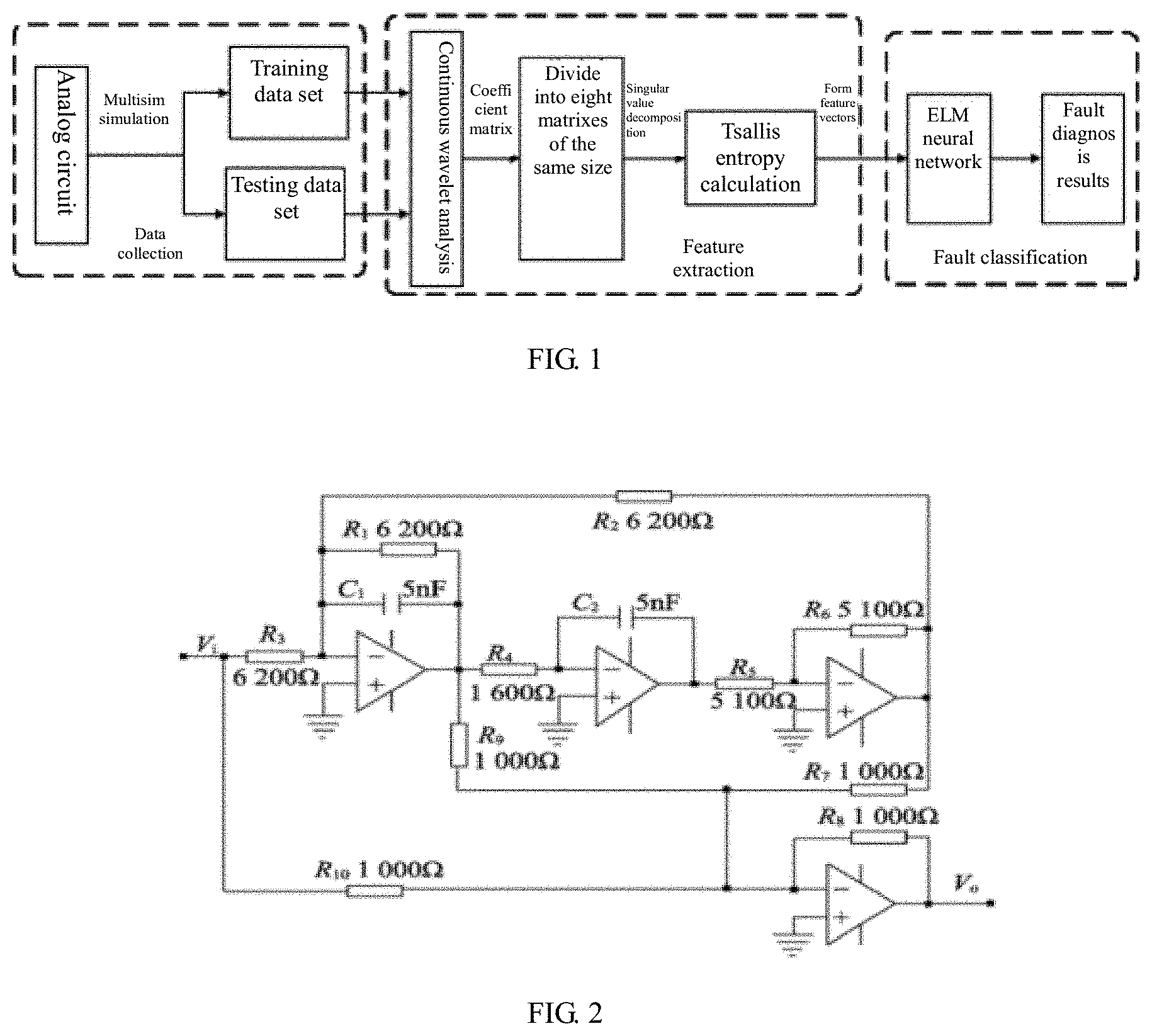
[0025] FIG. 2 is a circuit diagram of a four-operation-amplifier low-pass filter;
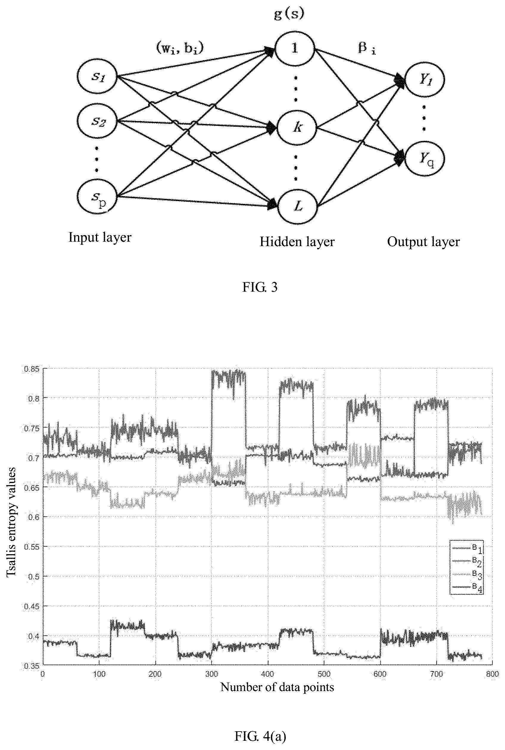
[0026] FIG. 3 is a structural diagram of an ELM network;
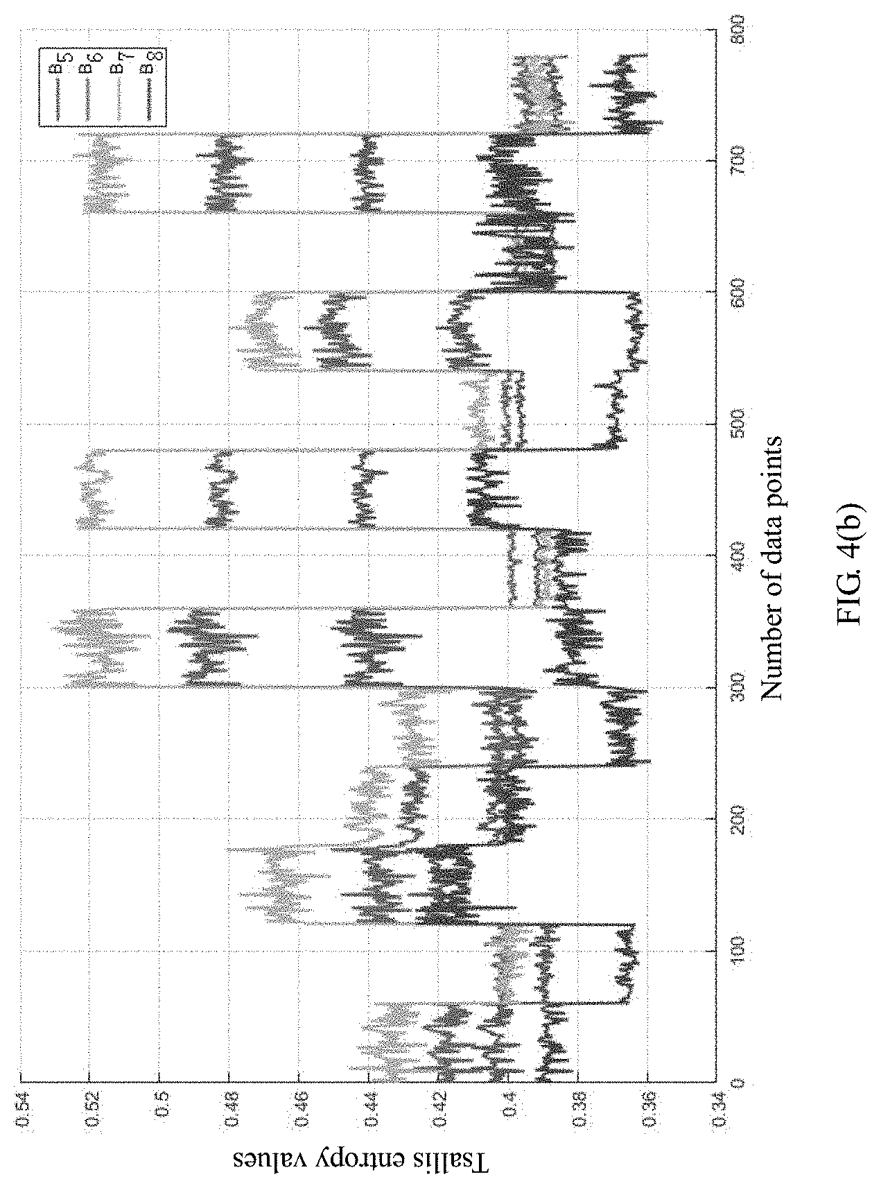
[0027] FIG. 4(a) is a diagram showing the Tsallis entropy fault features of sub-matrixes B.sub.1,B.sub.2,B.sub.3,B.sub.4 of a four-operation-amplifier low-pass filter;
[0028] FIG. 4(b) is a diagram showing the Tsallis entropy fault features of sub-matrixes B.sub.5,B.sub.6,B.sub.7,B.sub.8 of the four-operation-amplifier low-pass filter; and
[0029] FIG. 5 is a fault classification diagram of the four-operation-amplifier low-pass filter.
DETAILED DESCRIPTION OF THE INVENTION
[0030] The invention will be further described in detail below in conjunction with the accompanying drawings and particular embodiments.
[0031] 1. Fault Diagnosis Method
[0032] As shown in FIG. 1, the specific steps of the analog-circuit fault diagnosis method based on a continuous wavelet transform and an ELM network are as follows:
[0033] data acquisition: performing a data sampling on output responses of an analog circuit through Multisim simulation to obtain an output response data set;
[0034] feature extraction: performing a continuous wavelet transform by taking the output response data set of the circuit obtained through simulation, as a training data set and a testing data set to obtain a wavelet time-frequency coefficient matrix of fault signals, dividing the coefficient matrix into eight sub-matrixes of the same size, performing a singular value decomposition on the respective sub-matrixes to obtain singular values, and calculating a Tsallis entropy for the singular values of each sub-matrix, the Tsallis entropy values form corresponding circuit response fault feature vectors; and
[0035] fault classification: inputting the circuit response fault feature vectors into an ELM network to implement the accurate and quick fault classification.
[0036] The core technologies, i.e., continuous wavelet analysis, singular value decomposition, Tsallis entropy and ELM neural network, in the fault diagnosis method of the invention will be further illustrated in detail below.
[0037] 1.1 Continuous Wavelet Analysis
[0038] The continuous wavelet analysis originates from wavelet analysis. Continuous wavelets are characterized by continuously changing scales, and capable of more finely describing the local form of a signal. Continuous wavelet transform coefficients of a circuit response x(t) can be represented with the formula below:
W.sub.x(.tau.,a)= {square root over (a)}.intg..sub.-.infin..sup.+.infin.x(t).phi.(a(t-.tau.))dt=<x,.phi..s- ub..tau.,a> (1),
[0039] here, W.sub.x(.tau.,a) is a continuous wavelet transform time-frequency coefficient matrix; .tau. is a time parameter, and a is a frequency parameter, with a>0; .phi.(t) is a wavelet generating function; .phi..sub..tau.,a(t) is a wavelet basis function which is a set of function series formed by dilation and translation of the wavelet generating function .phi.(t), that is,
.PHI. .tau. , a ( t ) = 1 a .PHI. ( t - .tau. a ) . ( 2 ) ##EQU00005##
[0040] The continuous wavelet transform maps the signals to a time-frequency plane by means of the continuously changing time and scale, and the coefficient matrix W.sub.x(.tau., a) measures the level of similarity between the signals and wavelets, reflecting the feature information of the signals.
[0041] 1.2 Singular Value Decomposition and Tsallis Entropy Calculation
[0042] First, the time-frequency coefficient matrix W.sub.x(.tau.,a) obtained is equally divided into eight ft-actions, that is, the eight sub-matrixes B.sub.1,B.sub.2,B.sub.3,B.sub.4,B.sub.5,B.sub.6,B.sub.7,B.sub.8 are obtained according to
W x ( .tau. , a ) = [ ( B 1 ) m 2 .times. n 4 ( B 2 ) m 2 .times. n 4 ( B 3 ) m 2 .times. n 4 ( B 4 ) m 2 .times. n 4 ( B 5 ) m 2 .times. n 4 ( B 6 ) m 2 .times. n 4 ( B 7 ) m 2 .times. n 4 ( B 8 ) m 2 .times. n 4 ] m .times. n . ( 3 ) ##EQU00006##
According to the theory of singular value decomposition, the sub-matrixes are decomposed as follows:
B.sub.c.times.d=U.sub.c.times.lA.sub.l.times.lV.sub.l.times.d (4),
[0043] here, B.sub.c.times.d represents c.times.d-dimension sub-matrixes obtained after the division by the formula (3); and the principal diagonal elements .lamda..sub.i(i=1, 2, . . . , l) of a diagonal matrix A are the singular values of B.sub.c.times.d with .lamda..sub.1.gtoreq..lamda..sub.2 . . . .gtoreq..lamda..sub.l.gtoreq.0. l is the number of non-zero singular values of the matrix B.sub.c.times.d.
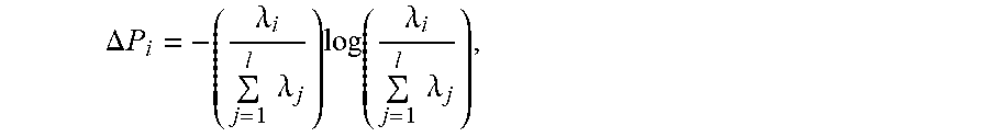
[0044] Said calculating a Tsallis entropy for the singular values of each sub-matrix is represented by the following formula:
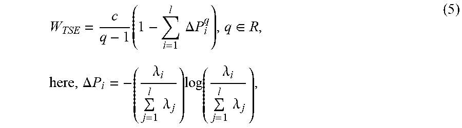
W TSE = c q - 1 ( 1 - i = 1 l .DELTA. P i q ) , q .di-elect cons. R , here , .DELTA. P i = - ( .lamda. i j = 1 l .lamda. j ) log ( .lamda. i j = 1 l .lamda. j ) , ( 5 ) ##EQU00007##
and q is a non-extensive parameter, with C=1 and q=1.2.
[0045] The Tsallis entropy values of the singular values of respective sub-matrixes as calculated with the formula (5) are combined together to form corresponding circuit response fault feature vectors.
[0046] 1.3 ELM Neural Network
[0047] The extreme learning machine is a new neural network based on single-hidden layer feed forward networks, which have been widely applied in practice due to their high learning speed and simple network structure. Research has shown that for the single-hidden layer feed forward networks, there is no need to either adjust the randomly initialized w.sub.i and b.sub.i or deviate the output layer as long as an excitation function g(s) is infinitely derivable in any real number interval, the output weight value .beta.i is calculated with a regularization principle to approach any continuous system, and there is almost no need to learn.
[0048] The ELM network lacks the output layer deviation, moreover, the input weight w and the hidden layer deviation b.sub.i are generated randomly and need no adjustment, only the output weight .beta..sub.i in the whole network needs to be determined.
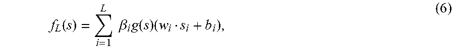
[0049] For each neuron in FIG. 3, the output of the ELM network can be uniformly represented in model as follows:
f L ( s ) = i = 1 L .beta. i g ( s ) ( w i s i + b i ) , ( 6 ) ##EQU00008##
[0050] here, s.sub.i=[s.sub.i1, s.sub.i2, . . . , s.sub.ip].sup.T R.sup.p,w.sub.i R.sup.p,.beta..sub.i R.sup.q, s is an input feature vector; p is the number of network input nodes, that is the dimension of the input feature vector; q is the number of network output node; L represents hidden layer nodes; and g(s) represents an excitation function. w.sub.i=[w.sub.i1, w.sub.i2, . . . , w.sub.ip].sup.T represents the input weights from the input layer to the i th hidden layer node; b.sub.i represents the deviation of the i th hidden node; and .beta..sub.i=[.beta..sub.i1, .beta..sub.i2, . . . , .beta..sub.iq].sup.T is the output weight connecting the i th hidden layer node.
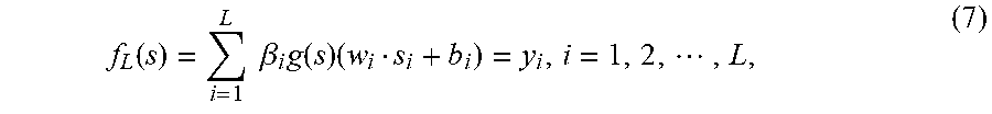
[0051] When the feed forward neural network having L hidden layer nodes can approach the sample with zero error, then w.sub.i, b.sub.i and .beta..sub.i exist, allowing:
f L ( s ) = i = 1 L .beta. i g ( s ) ( w i s i + b i ) = y i , i = 1 , 2 , , L , ( 7 ) ##EQU00009##
here, y.sub.i=[y.sub.i1, y.sub.i2, . . . , y.sub.ip].sup.T R.sup.q represents the output of the network.
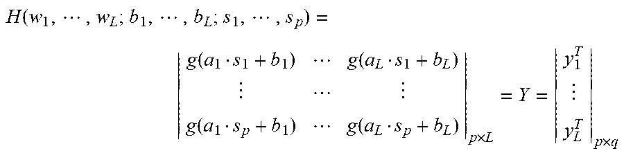
[0052] The formula (7) can be simplified into H.beta.=Y, wherein,
H ( w 1 , , w L ; b 1 , , b L ; s 1 , , s p ) = g ( a 1 s 1 + b 1 ) g ( a L s 1 + b L ) g ( a 1 s p + b 1 ) g ( a L s p + b L ) p .times. L = Y = y 1 T y L T p .times. q ##EQU00010##
[0053] here, p is the number of network input nodes, that is, the dimension of the input feature vector; q is the number of network output node;
[0054] H represents the hidden layer output matrix of the network, and the output weight matrix can be obtained from the formula below:
.beta.=H.sup.+Y (8),
[0055] here, H.sup.+ is a Moore-Penrose generalized inverse matrix of H.
[0056] 2. Exemplary Circuit and Method Application:
[0057] FIG. 2 shows a four-operation-amplifier biquad high-pass filter, with the nominal values of respective elements marked in the figure. By taking this circuit as an example, the whole process flow of the fault diagnosis method provided by the invention is demonstrated, where pulse waves with the duration of 10 us and the amplitude of 10V are used as an excitation source, and fault time-domain response signals are obtained at the output end of the circuit. The tolerance range of the circuit elements is set as 5%.
[0058] R1, R2, R3, R4, C1 and C2 are selected as test objects, and Table 1 gives the fault code, fault type, nominal value and fault value of each circuit element under test, where .uparw. and .dwnarw. represent being above and below the nominal value respectively, and NF represents no fault. 60 data are sampled for each of the fault types respectively and divided into two parts, the former 30 data are used to establish the ELM network fault diagnosis model based on continuous wavelet transform, and the latter 30 data are used to test the performance of this fault diagnosis model.
TABLE-US-00001 TABLE 1 Fault code, fault type, nominal value and fault value Fault Code Fault Type Nominal Value Fault Value F0 NF F1 R1.dwnarw. 6200.OMEGA. 3000.OMEGA. F2 R1.uparw. 6200.OMEGA. 15000.OMEGA. F3 R2.dwnarw. 6200.OMEGA. 2000.OMEGA. F4 R2.uparw. 6200.OMEGA. 18000.OMEGA. F5 R3.dwnarw. 6200.OMEGA. 2700.OMEGA. F6 R3.uparw. 6200.OMEGA. 12000.OMEGA. F7 R4.dwnarw. 1600.OMEGA. 500.OMEGA. F8 R4.uparw. 1600.OMEGA. 2500.OMEGA. F9 C1.dwnarw. 5 nF 2.5 nF F10 C1.uparw. 5 nF 10 nF F11 C2.dwnarw. 5 nF 1.5 nF F12 C2.uparw. 5 nF 15 nF
[0059] Data Acquisition:
[0060] In the four-operation-amplifier biquad high-pass filter, the applied excitation response is a pulse sequence with the amplitude of 10V and the duration of 10 us. The output response of the circuit under different fault modes is subjected to Multisim simulation.
[0061] Feature Extraction:
[0062] The continuous wavelet transform is used below to analyze the output responses of the circuit, where the complex Morlet wavelet is selected as the wavelet basis for wavelet analysis. The output response coefficient matrix obtained is divided into eight sub-matrixes, which are then subjected to singular value decomposition according to the formulae (4) and (5) for calculating Tsallis entropy features.
[0063] As is known, the greater the feature value difference among different faults or between the faults and the normal status, the more significant the signal response difference among different faults or between the faults and the normal status, and the more beneficial this fault feature is to the fault diagnosis. As can be known from FIGS. 4(a) and 4(b), the numeric difference between the response features of the circuit in fault and the response features of the circuit in normal status as obtained with the method of the invention, as well as the numeric differences of the features of the circuit under different fault modes are significant, which fully demonstrate the effectiveness of the fault feature extraction of the invention.
[0064] Fault Classification:
[0065] The Tsallis entropy feature set obtained is divided into two parts, i.e., a training set and a testing set. The training set is input into the ELM network to train the ELM classifier model, and after the completion of the training, the testing set is input into the ELM classifier model, with the fault diagnosis results as shown in FIG. 5. The ELM classifier model successfully identifies all the faults, with the overall success rate up to 100% for the fault diagnosis.
* * * * *
D00000
D00001
D00002
D00003
D00004


XML
uspto.report is an independent third-party trademark research tool that is not affiliated, endorsed, or sponsored by the United States Patent and Trademark Office (USPTO) or any other governmental organization. The information provided by uspto.report is based on publicly available data at the time of writing and is intended for informational purposes only.
While we strive to provide accurate and up-to-date information, we do not guarantee the accuracy, completeness, reliability, or suitability of the information displayed on this site. The use of this site is at your own risk. Any reliance you place on such information is therefore strictly at your own risk.
All official trademark data, including owner information, should be verified by visiting the official USPTO website at www.uspto.gov. This site is not intended to replace professional legal advice and should not be used as a substitute for consulting with a legal professional who is knowledgeable about trademark law.