Precoding In Wireless Systems Using Orthogonal Time Frequency Space Multiplexing
A1
U.S. patent application number 16/859135 was filed with the patent office on 2020-08-13 for precoding in wireless systems using orthogonal time frequency space multiplexing. The applicant listed for this patent is Cohere Technologies, Inc.. Invention is credited to James Delfeld.
| Application Number | 20200259697 16/859135 |
| Document ID | 20200259697 / US20200259697 |
| Family ID | 1000004829334 |
| Filed Date | 2020-08-13 |
| Patent Application | download [pdf] |

View All Diagrams
| United States Patent Application | 20200259697 |
| Kind Code | A1 |
| Delfeld; James | August 13, 2020 |
PRECODING IN WIRELESS SYSTEMS USING ORTHOGONAL TIME FREQUENCY SPACE MULTIPLEXING
Abstract
Device, methods and systems for recoding in wireless systems using orthogonal time frequency space multiplexing are described. An exemplary method for transmitting wireless signals includes mapping data to generate a quadrature amplitude modulation (QAM) signal in a delay Doppler domain, determining a perturbation signal to minimize expected interference and noise, perturbing the QAM signal with the perturbation signal, thereby producing a perturbed signal, generating a pre-coded signal by pre-coding, using a linear pre-coder, the perturbed signal, and transmitting the pre-coded signal using an orthogonal time frequency space modulation signal scheme.
| Inventors: | Delfeld; James; (Santa Clara, CA) | ||||||||||
| Applicant: |
|
||||||||||
|---|---|---|---|---|---|---|---|---|---|---|---|
| Family ID: | 1000004829334 | ||||||||||
| Appl. No.: | 16/859135 | ||||||||||
| Filed: | April 27, 2020 |
Related U.S. Patent Documents
| Application Number | Filing Date | Patent Number | ||
|---|---|---|---|---|
| PCT/US2018/058787 | Nov 1, 2018 | |||
| 16859135 | ||||
| 62580047 | Nov 1, 2017 | |||
| 62587289 | Nov 16, 2017 | |||
| Current U.S. Class: | 1/1 |
| Current CPC Class: | H04B 7/0421 20130101; H04L 27/34 20130101; H04B 7/0456 20130101 |
| International Class: | H04L 27/34 20060101 H04L027/34; H04B 7/0456 20060101 H04B007/0456; H04B 7/0417 20060101 H04B007/0417 |
Claims
1. A method for transmitting a wireless signal, comprising: mapping a plurality of data bits to generate a quadrature amplitude modulation (QAM) signal in a delay-Doppler domain; determining a perturbation signal to minimize expected interference and noise; perturbing the QAM signal with the perturbation signal to produce a first perturbed signal; transforming, using a two-dimensional (2D) Fourier transform, the first perturbed signal into a second perturbed signal from the delay-Doppler domain to a time-frequency domain; generating a pre-coded signal by pre-coding, using a linear pre-coder, the second perturbed signal; and transmitting the pre-coded signal using an orthogonal time frequency space (OTFS) modulation signal scheme.
2. The method of claim 1, wherein the pre-coded signal is spatially selective such that a greater energy is emitted in a first direction for which a first channel state information (CSI) estimate is available than a second direction for which a second CSI estimate is available, and wherein the second CSI estimate is less accurate than the first CSI estimate.
3. The method of claim 1, further including: updating the linear pre-coder using an explicit feedback from a user device.
4. The method of claim 1, further including: updating the linear pre-coder using an implicit feedback.
5. The method of claim 1, wherein the determining the perturbation signal includes: selecting, as the perturbation signal, a set of lattice points of a coarse lattice structure.
6. The method of claim 5, wherein the selecting comprises using a non-linear filter to select the set of lattice points that minimizes the expected interference and noise, and wherein the non-linear filter comprises a Tomlinson-Harashima filter.
7. (canceled)
8. The method of claim 1, wherein the selecting the perturbation signal includes selecting p.sub.opt, that minimizes: f = 1 N f t = 1 N t ( X ( f , t ) + P ( f , t ) ) * M error ( f , t ) ( X ( f , t ) + P ( f , t ) ) , ##EQU00066## wherein f and t are integer variables, N.sub.f and N.sub.t represent frequency bins and time bins, respectively, X(f,t) is a two-dimensional representation of an input signal in time and frequency domains, P(f,t) is a two-dimensional representation of the perturbation signal in time and frequency domains, * represents a conjugation operation, and M.sub.error(f,t) represents an error metric.
9. The method of claim 1, wherein the linear pre-coder is based on an estimate of a wireless channel over which the pre-coded signal is transmitted.
10. (canceled)
11. (canceled)
12. A method for receiving a wireless communication, including: receiving a quadrature amplitude modulation (QAM) signal in a time-frequency domain; applying an orthogonal transformation to convert the received QAM signal from the time-frequency domain to a delay-Doppler domain; determining a closest lattice point corresponding to a QAM constellation point of the QAM signal in the delay-Doppler domain; removing a perturbation in the received QAM signal by subtracting the closest lattice point from the QAM constellation point to generate an un-perturbed QAM signal; and demodulating the un-perturbed QAM signal to obtain a plurality of data bits.
13. The method of claim 12, wherein the determining the closest lattice point comprises projecting the received QAM signal in the delay-Doppler domain onto a coarse lattice structure, and wherein the perturbation lies on the coarse lattice structure.
14. The method of claim 12, wherein the determining the closest lattice point is based on using a non-linear filter to minimize an error associated with the received QAM signal.
15. The method of claim 14, wherein the non-linear filter comprises a spatial Tomlinson-Harashima filter.
16. The method of claim 14, wherein the QAM signal is received through a wireless channel, and wherein the non-linear filter is based on estimated second order statistics of the wireless channel.
17. (canceled)
18. (canceled)
19. The method of 12, wherein the determining the closest lattice point comprises minimizing the quadratic form argmin p .di-elect cons. ( 2 + 2 j ) L u ( r ( .tau. ) + p ) * D ( .tau. ) ( r ( .tau. ) + p ) ##EQU00067## wherein p is the perturbation, r(.tau.) is the received QAM signal in the delay-Doppler domain, L.sub.u, is a length of a transmitted QAM signal corresponding to the plurality of data bits, 2+2j is a coarse lattice structure, and D(.tau.) is a .tau.-th block diagonal entry of a positive definite block diagonal matrix corresponding to a Cholesky decomposition of the perturbation.
20. An apparatus for wireless communication, comprising: a processor; and a transceiver circuitry coupled to the processor, wherein the transceiver circuitry is configured to: receive a quadrature amplitude modulation (QAM) signal in a time-frequency domain, and wherein the processor is configured to: apply an orthogonal transformation to convert the received QAM signal from the time-frequency domain to a delay-Doppler domain, determine a closest lattice point corresponding to a QAM constellation point of the QAM signal in the delay-Doppler domain, remove a perturbation in the received QAM signal by subtracting the closest lattice point from the QAM constellation point to generate an un-perturbed QAM signal, and demodulate the un-perturbed QAM signal to obtain a plurality of data bits.
21. The apparatus of claim 20, wherein determining the closest lattice point comprises projecting the received QAM signal in the delay-Doppler domain onto a coarse lattice structure, and wherein the perturbation lies on the coarse lattice structure.
22. The apparatus of claim 20, wherein the determining the closest lattice point is based on using a non-linear filter to minimize an error associated with the received QAM signal.
23. The apparatus of claim 22, wherein the non-linear filter comprises a spatial Tomlinson-Harashima filter.
24. The apparatus of claim 22, wherein the QAM signal is received through a wireless channel, and wherein the non-linear filter is based on estimated second order statistics of the wireless channel.
25. The apparatus of 20, wherein the determining the closest lattice point comprises minimizing the quadratic form argmin p .di-elect cons. ( 2 + 2 j ) L u ( r ( .tau. ) + p ) * D ( .tau. ) ( r ( .tau. ) + p ) ##EQU00068## wherein p is the perturbation, r(.tau.) is the received QAM signal in the delay-Doppler domain, L.sub.u is a length of a transmitted QAM signal corresponding to the plurality of data bits, 2Z+2j is a coarse lattice structure, and D(.tau.) is a .tau.-th block diagonal entry of a positive definite block diagonal matrix corresponding to a Cholesky decomposition of the perturbation.
Description
CROSS-REFERENCES TO RELATED APPLICATIONS
[0001] This patent document claims priority to and benefits of U.S. Provisional Application No. 62/580,047 entitled "PRECODING IN ORTHOGONAL TIME FREQUENCY SPACE MULTIPLEXING" filed on 1 Nov. 2017, and U.S. Provisional Application No. 62/587,289 entitled "PRECODING IN ORTHOGONAL TIME FREQUENCY SPACE MULTIPLEXING" filed on 16 Nov. 2017. The entire contents of the aforementioned patent applications are incorporated by reference as part of the disclosure of this patent document.
TECHNICAL FIELD
[0002] The present document relates to wireless communication, and more particularly, to using precoding in wireless communications.
BACKGROUND
[0003] Due to an explosive growth in the number of wireless user devices and the amount of wireless data that these devices can generate or consume, current wireless communication networks are fast running out of bandwidth to accommodate such a high growth in data traffic and provide high quality of service to users.
[0004] Various efforts are underway in the telecommunication industry to come up with next generation of wireless technologies that can keep up with the demand on performance of wireless devices and networks.
SUMMARY
[0005] This document discloses techniques that can be used to precode wireless signals.
[0006] In one example aspect, a method for transmitting wireless signals is disclosed. The method includes mapping data to generate a quadrature amplitude modulation (QAM) signal in a delay Doppler domain, determining a perturbation signal to minimize expected interference and noise, perturbing the QAM signal with the perturbation signal, thereby producing a perturbed signal, generating a pre-coded signal by pre-coding, using a linear pre-coder, the perturbed signal, and transmitting the pre-coded signal using an orthogonal time frequency space modulation signal scheme.
[0007] In another example aspect, a wireless communication method is disclosed. The method includes generating a quadrature amplitude modulation (QAM) signal in the 2D delay-Doppler domain by modulating data bits, using an error metric along with the QAM signal to generate a perturbation signal, adding the perturbation signal to the QAM signal to generate a perturbed QAM signal, transforming the perturbed QAM signal into the 2D time frequency domain by using a 2D Fourier transform from the 2D delay Doppler domain to the 2D time frequency domain, filtering the 2D transformed signal using an optimal precoding filter to generate a precoded signal, and transmitting the precoded signal over a communication medium.
[0008] In yet another example aspect, a method of receiving wireless signals is disclosed. The method includes receiving a quadrature amplitude modulation (QAM) signal in the time-frequency domain, applying an orthogonal transformation to convert the received QAM signal into delay-Doppler domain, determining a closest lattice point corresponding to the QAM constellation point of the QAM signal in the delay-Doppler domain, removing perturbation in the received QAM signal by subtracting the closest lattice point from the QAM constellation point, and demodulating the un-perturbed QAM signal to obtain data.
[0009] In another example aspect, a wireless communication apparatus that implements the above-described methods is disclosed.
[0010] In yet another example aspect, the method may be embodied as processor-executable code and may be stored on a computer-readable program medium.
[0011] These, and other, features are described in this document.
DESCRIPTION OF THE DRAWINGS
[0012] Drawings described herein are used to provide a further understanding and constitute a part of this application. Example embodiments and illustrations thereof are used to explain the technology rather than limiting its scope.
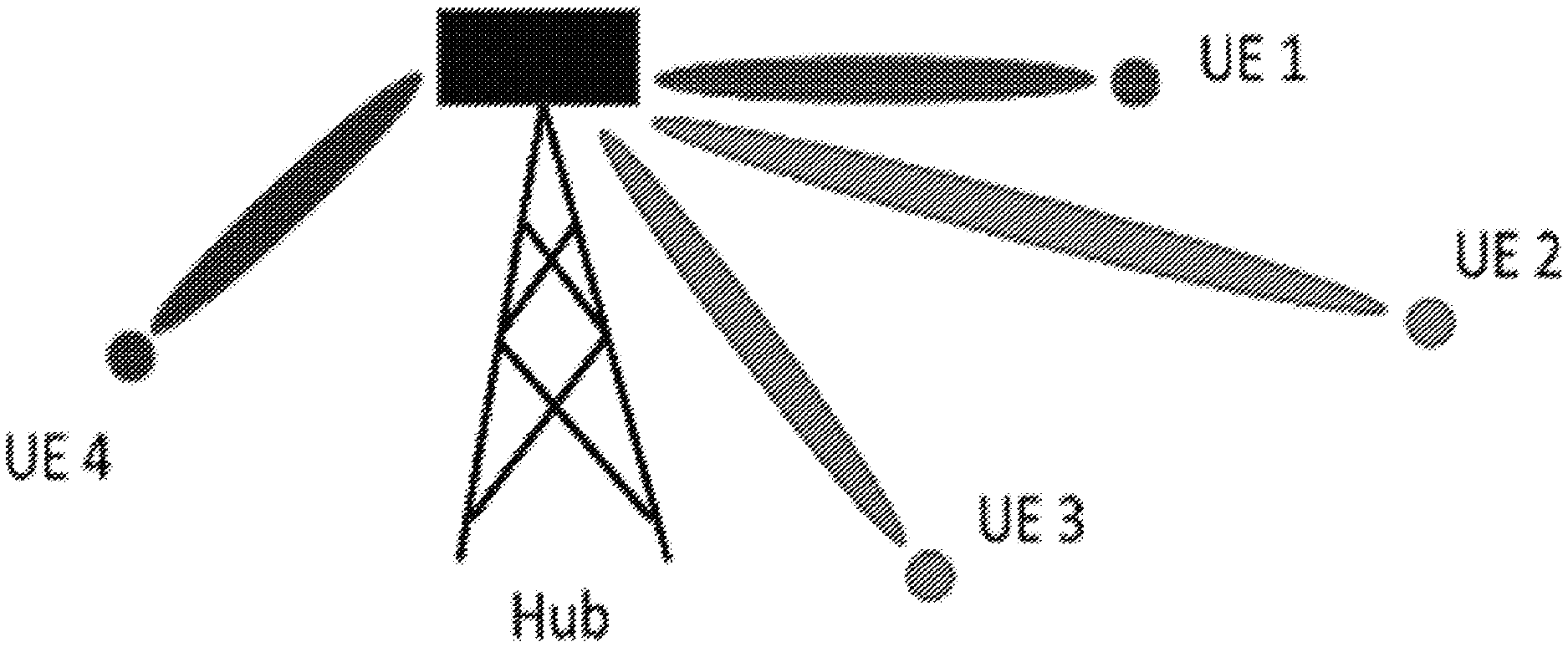
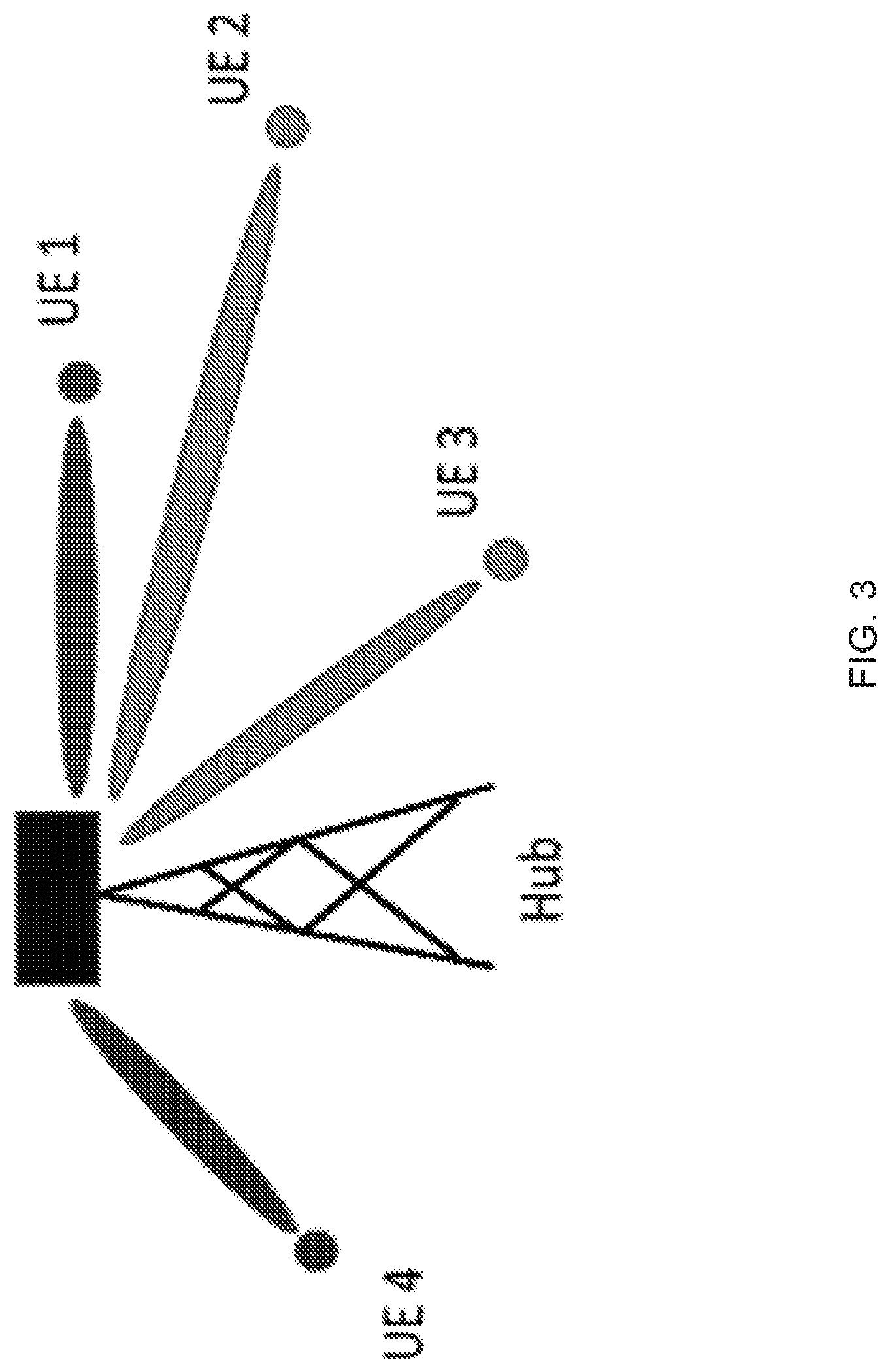
[0013] FIG. 1 depicts an example network configuration in which a hub services for user equipment (UE).
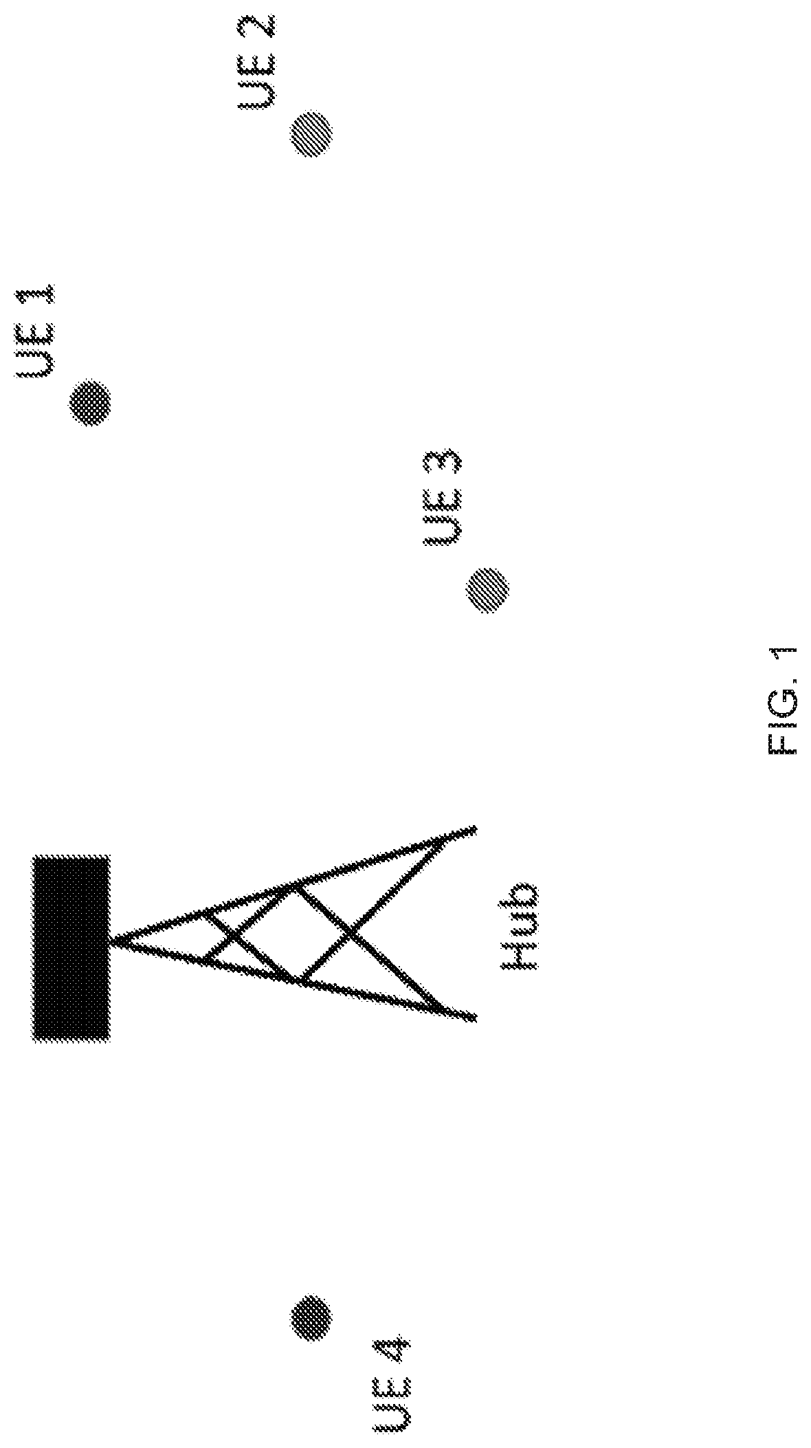
[0014] FIG. 2 depicts an example embodiment in which an orthogonal frequency division multiplexing access (OFDMA) scheme is used for communication.
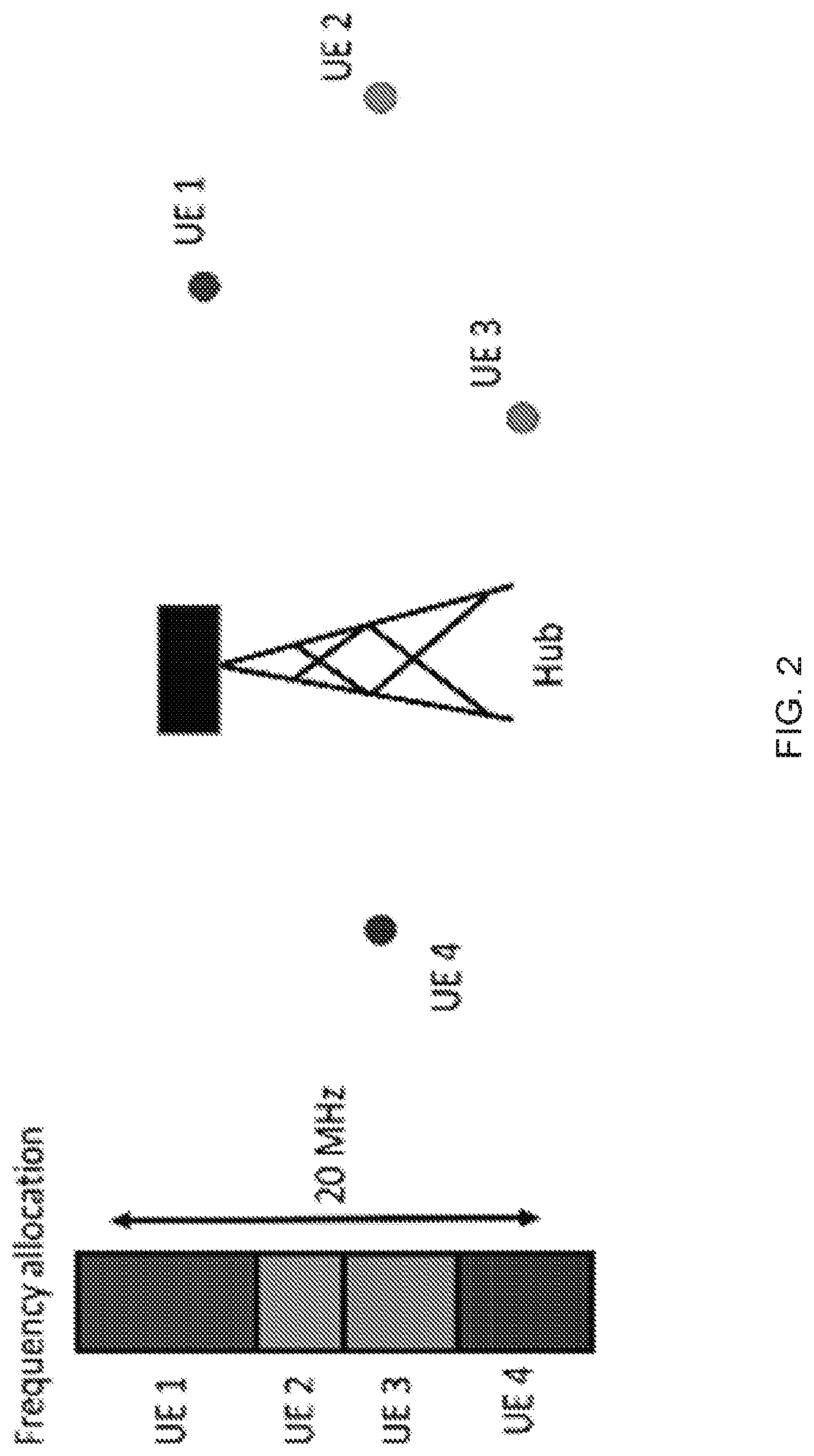
[0015] FIG. 3 illustrates the concept of precoding in an example network configuration.
[0016] FIG. 4 is a spectral chart of an example of a wireless communication channel.
[0017] FIG. 5 illustrates examples of downlink and uplink transmission directions.
[0018] FIG. 6 illustrates spectral effects of an example of a channel prediction operation.
[0019] FIG. 7 graphically illustrates operation of an example implementation of a zero-forcing precoder (ZFP).
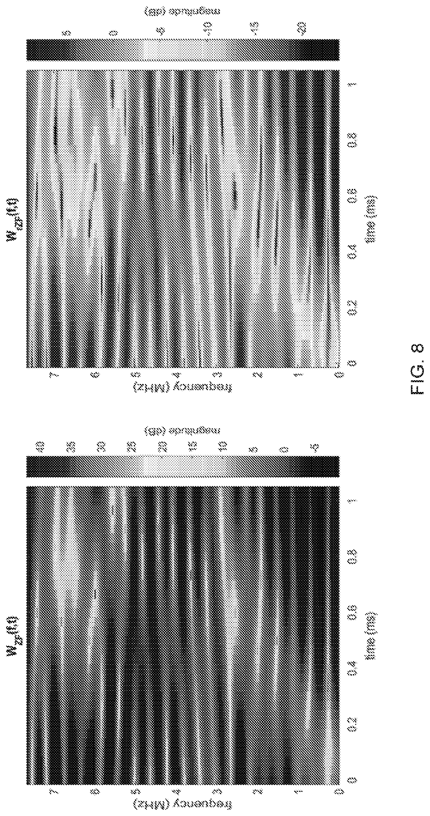
[0020] FIG. 8 graphically compares two implementations--a ZFP implementation and regularized ZFP implementation (rZFP).
[0021] FIG. 9 shows components of an example embodiment of a precoding system.
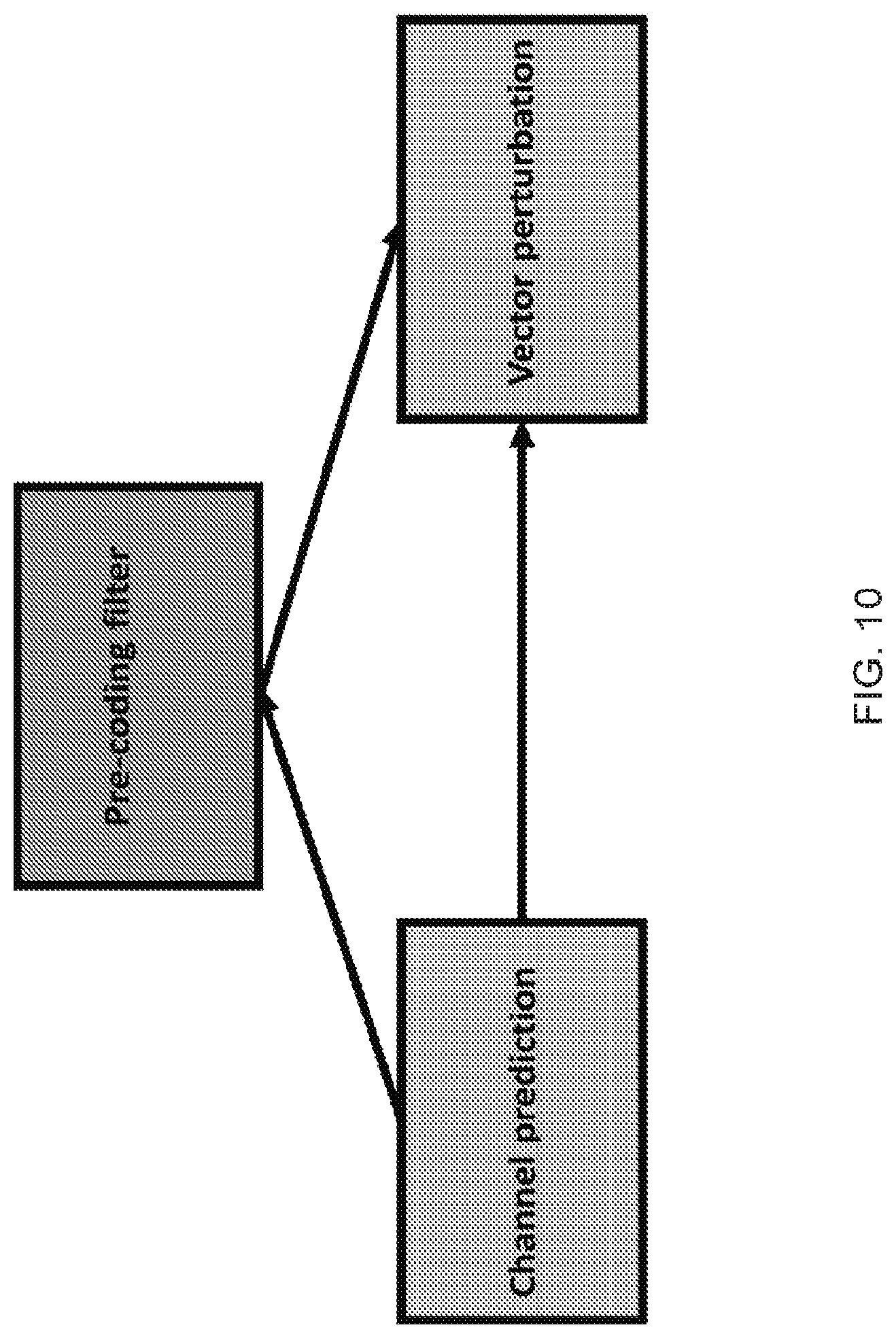
[0022] FIG. 10 is a block diagram depiction of an example of a precoding system.
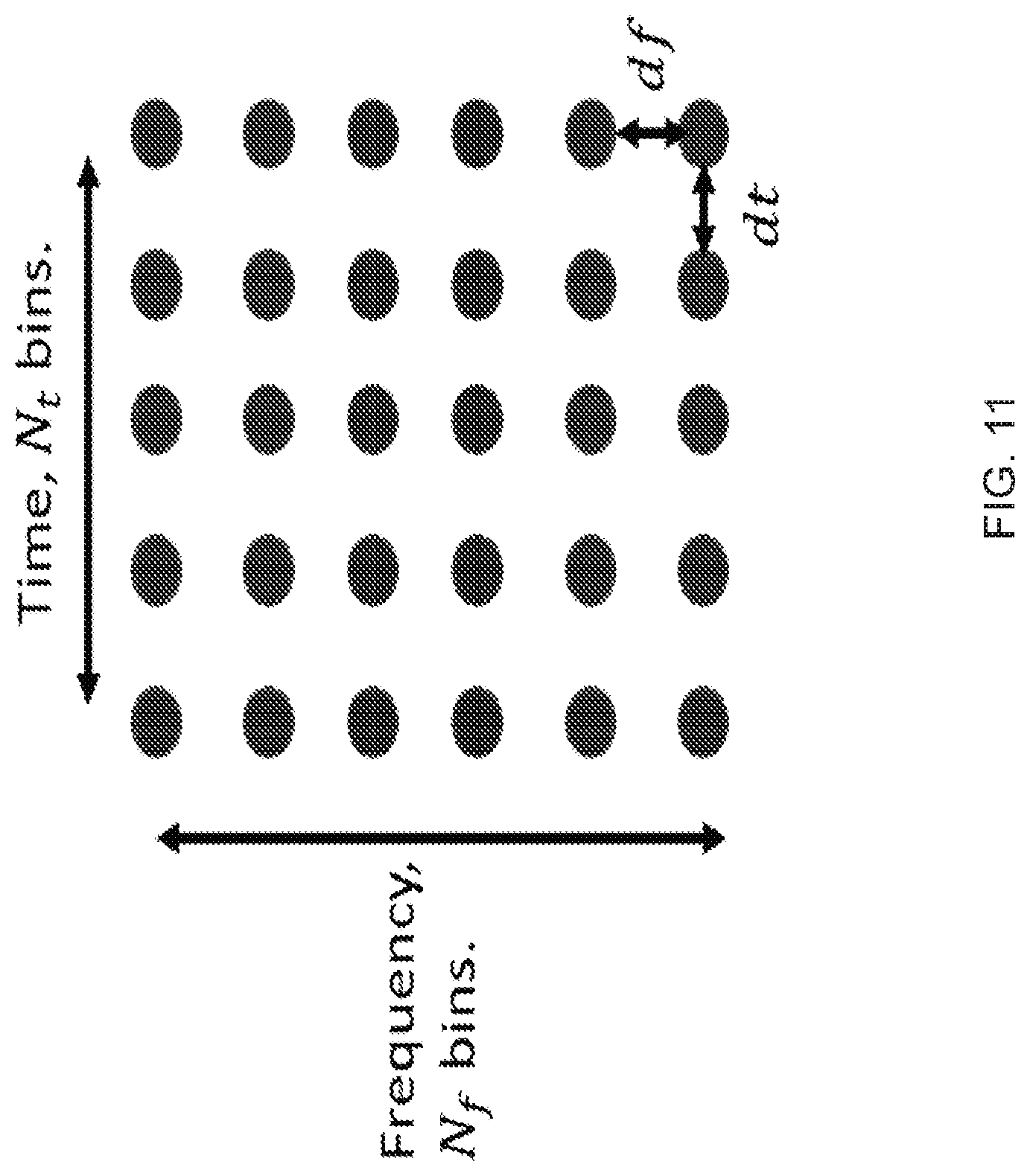
[0023] FIG. 11 shows an example of a quadrature amplitude modulation (QAM) constellation.
[0024] FIG. 12 shows another example of QAM constellation.
[0025] FIG. 13 pictorially depicts an example of relationship between delay-Doppler domain and time-frequency domain.
[0026] FIG. 14 is a spectral graph of an example of an extrapolation process.
[0027] FIG. 15 is a spectral graph of another example of an extrapolation process.
[0028] FIG. 16 compares spectra of a true and a predicted channel in some precoding implementation embodiments.
[0029] FIG. 17 is a block diagram depiction of a process for computing prediction filter and error covariance.
[0030] FIG. 18 is a block diagram illustrating an example of a channel prediction process.
[0031] FIG. 19 is a graphical depiction of channel geometry of an example wireless channel.
[0032] FIG. 20 is a graph showing an example of a precoding filter antenna pattern.
[0033] FIG. 21 is a graph showing an example of an optical pre-coding filter.
[0034] FIG. 22 is a block diagram showing an example process of error correlation computation.
[0035] FIG. 23 is a block diagram showing an example process of precoding filter estimation.
[0036] FIG. 24 is a block diagram showing an example process of applying an optimal precoding filter.
[0037] FIG. 25 is a graph showing an example of a lattice and QAM symbols.
[0038] FIG. 26 graphically illustrates effects of perturbation examples.
[0039] FIG. 27 is a graph illustrating an example of hub transmission.
[0040] FIG. 28 is a graph showing an example of the process of a UE finding a closest coarse lattice point.
[0041] FIG. 29 is a graph showing an example process of UE recovering a QPSK symbol by subtraction.
[0042] FIG. 30 depicts an example of a channel response.
[0043] FIG. 31 depicts an example of an error of channel estimation.
[0044] FIG. 32 shows a comparison of energy distribution of an example of QAM signals and an example of perturbed QAM signals.
[0045] FIG. 33 is a graphical depiction of a comparison of an example error metric with an average perturbed QAM energy.
[0046] FIG. 34 is a block diagram illustrating an example process of computing an error metric.
[0047] FIG. 35 is a block diagram illustrating an example process of computing perturbation.
[0048] FIG. 36 is a block diagram illustrating an example of application of a precoding filter.
[0049] FIG. 37 is a block diagram illustrating an example process of UE removing the perturbation.
[0050] FIG. 38 is a block diagram illustrating an example spatial Tomlinsim Harashima precoder (THP).
[0051] FIG. 39 is a spectral chart of the expected energy error for different PAM vectors.
[0052] FIG. 40 is a plot illustrating an example result of a spatial THP.
[0053] FIG. 41 shows examples of local signals in delay-Doppler domain being non-local in time-frequency domain
[0054] FIG. 42 is a block diagram illustrating an example of the computation of coarse perturbation using Cholesky factor.
[0055] FIG. 43 shows an exemplary estimate of the channel impulse response for the SISO single carrier case.
[0056] FIG. 44 shows spectral plots of an example of the comparison of Cholesky factor and its inverse.
[0057] FIG. 45 shows an example of an overlay of U.sup.-1 column slices.
[0058] FIG. 46 is a block diagram illustrating an example of the computation of coarse perturbation using U.sup.-1 for the SISO single carrier case.
[0059] FIG. 47 is a block diagram illustrating an example of the computation of coarse perturbations using W.sub.THP for the SISO single carrier case.
[0060] FIG. 48 shows an exemplary plot of a channel frequency response for the SISO single carrier case.
[0061] FIG. 49 shows an exemplary plot comparing linear and non-linear precoders for the SISO single carrier case.
[0062] FIG. 50 is a block diagram illustrating an example of the algorithm for the computation of perturbation using U.sup.-1 for the SISO OTFS case.
[0063] FIG. 51 is a block diagram illustrating an example of the update step of the algorithm for the computation of perturbation using U.sup.-1 for the SISO OTFS case.
[0064] FIG. 52 shows an exemplary spectral plot of a channel frequency response for the SISO OTFS case.
[0065] FIG. 53 shows exemplary spectral plots comparing the SINR experienced by the UE for two precoding schemes for the SISO OTFS case.
[0066] FIG. 54 is a block diagram illustrating an example of the update step of the algorithm for the computation of perturbation using U.sup.-1 for the MIMO single carrier case.
[0067] FIG. 55 is a block diagram illustrating an example of the update step of the algorithm for the computation of perturbation using W.sub.THP for the MIMO single carrier case.
[0068] FIG. 56 shows plots comparing the SINR experienced by the 8 UEs for two precoding schemes in the MIMO single carrier case.
[0069] FIG. 57 is a block diagram illustrating an example of the update step of the algorithm for the computation of perturbation using U.sup.-1 for the MIMO OTFS case.
[0070] FIG. 58 is a block diagram illustrating an example of the update step of the algorithm for the computation of perturbation using W.sub.THP for the MIMO OTFS case.
[0071] FIG. 59 shows plots comparing the SINR experienced by 1 UE for two precoding schemes in the MIMO OTFS case.
[0072] FIG. 60 is a flowchart of an example wireless communication method.
[0073] FIG. 61 is a flowchart of an example wireless communication method.
[0074] FIG. 62 is a flowchart of an example wireless communication method.
[0075] FIG. 63 is an example of a wireless communication system.
[0076] FIG. 64 is a block diagram of a wireless communication apparatus.
DETAILED DESCRIPTION
[0077] To make the purposes, technical solutions and advantages of this disclosure more apparent, various embodiments are described in detail below with reference to the drawings. Unless otherwise noted, embodiments and features in embodiments of the present document may be combined with each other.
[0078] Section headings are used in the present document, including the appendices, to improve readability of the description and do not in any way limit the discussion to the respective sections only. The terms "hub" and user equipment/device are used to refer to the transmitting side apparatus and the receiving side apparatus of a transmission, and each may take the form of a base station, a relay node, an access point, a small-cell access point, user equipment, and so on.
[0079] Multiple Access
[0080] FIG. 1 depicts a typical example scenario in wireless communication is a hub transmitting data over a fixed time and bandwidth to several user devices (UEs). For example: a tower transmitting data to several cell phones, or a Wi-Fi router transmitting data to several devices. Such scenarios are called multiple access scenarios.
[0081] Orthogonal Multiple Access
[0082] Currently the common technique used for multiple access is orthogonal multiple access. This means that the hub breaks it's time and frequency resources into disjoint pieces and assigns them to the UEs. An example is shown in FIG. 2, where four UEs (UE1, UE2, UE3 and UE4) get four different frequency allocations and therefore signals are orthogonal to each other.
[0083] The advantage of orthogonal multiple access is that each UE experience its own private channel with no interference. The disadvantage is that each UE is only assigned a fraction of the available resource and so typically has a low data rate compared to non-orthogonal cases.
[0084] Precoding Multiple Access
[0085] Recently, a more advanced technique, precoding, has been proposed for multiple access. In precoding, the hub is equipped with multiple antennas. The hub uses the multiple antennas to create separate beams which it then uses to transmit data over the entire bandwidth to the UEs. An example is depicted in FIG. 3, which shows that the hub is able to form individual beams of directed RF energy to UEs based on their positions.
[0086] The advantage of precoding it that each UE receives data over the entire bandwidth, thus giving high data rates. The disadvantage of precoding is the complexity of implementation. Also, due to power constraints and noisy channel estimates the hub cannot create perfectly disjoint beams, so the UEs will experience some level of residual interference.
[0087] Introduction to Precoding
[0088] Precoding may be implemented in four steps: channel acquisition, channel extrapolation, filter construction, filter application.
[0089] Channel acquisition: To perform precoding, the hub determines how wireless signals are distorted as they travel from the hub to the UEs. The distortion can be represented mathematically as a matrix: taking as input the signal transmitted from the hubs antennas and giving as output the signal received by the UEs, this matrix is called the wireless channel.
[0090] Channel prediction: In practice, the hub first acquires the channel at fixed times denoted by s.sub.1, s.sub.2, . . . , s.sub.n. Based on these values, the hub then predicts what the channel will be at some future times when the pre-coded data will be transmitted, we denote these times denoted by t.sub.1, t.sub.2, . . . , t.sub.m.
[0091] Filter construction: The hub uses the channel predicted at t.sub.1, t.sub.2, . . . , t.sub.m to construct precoding filters which minimize the energy of interference and noise the UEs receive.
[0092] Filter application: The hub applies the precoding filters to the data it wants the UEs to receive.
[0093] Channel Acquisition
[0094] This section gives a brief overview of the precise mathematical model and notation used to describe the channel.
[0095] Time and frequency bins: the hub transmits data to the UEs on a fixed allocation of time and frequency. This document denotes the number of frequency bins in the allocation by N.sub.f and the number of time bins in the allocation by N.sub.t.
[0096] Number of antennas: the number of antennas at the hub is denoted by L.sub.h, the total number of UE antennas is denoted by L.sub.u.
[0097] Transmit signal: for each time and frequency bin the hub transmits a signal which we denote by .phi.(f,t).di-elect cons..sup.L.sup.h for f=1, . . . , N.sub.f and t=1, . . . , N.sub.t.
[0098] Receive signal: for each time and frequency bin the UEs receive a signal which we denote by y(f,t).di-elect cons..sup.L.sup.u for f=1, . . . , N.sub.f and t=1, . . . , N.sub.t.
[0099] White noise: for each time and frequency bin white noise is modeled as a vector of iid Gaussian random variables with mean zero and variance N.sub.0. This document denotes the noise by w(f,t).di-elect cons..sup.L.sup.u for f=1, . . . , N.sub.f and t=1, . . . , N.sub.t.
[0100] Channel matrix: for each time and frequency bin the wireless channel is represented as a matrix and is denoted by H(f,t).di-elect cons..sup.L.sup.u.sup..times.L.sup.h for f=1, . . . , N.sub.f and t=1, . . . , N.sub.t.
[0101] The wireless channel can be represented as a matrix which relates the transmit and receive signals through a simple linear equation:
y(f,t)=H(f,t).phi.(f,t)+w(f,t) (1)
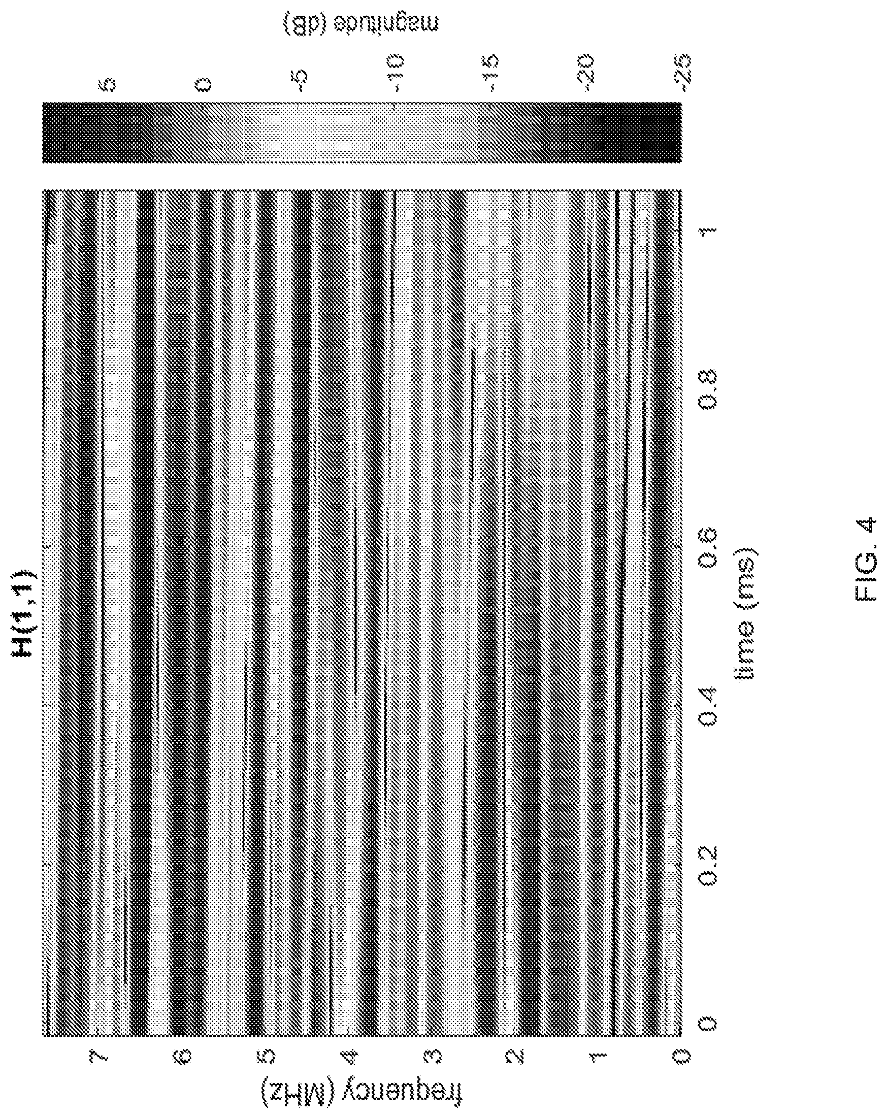
[0102] for f=1, . . . ,N.sub.f and t=1, . . . , N.sub.t. FIG. 4 shows an example spectrogram of a wireless channel between a single hub antenna and a single UE antenna. The graph is plotted with time as the horizontal axis and frequency along the vertical axis. The regions are shaded to indicate where the channel is strong or weak, as denoted by the dB magnitude scale shown in FIG. 4.
[0103] Two common ways are typically used to acquire knowledge of the channel at the hub: explicit feedback and implicit feedback.
[0104] Explicit Feedback
[0105] In explicit feedback, the UEs measure the channel and then transmit the measured channel back to the hub in a packet of data. The explicit feedback may be done in three steps.
[0106] Pilot transmission: for each time and frequency bin the hub transmits a pilot signal denoted by p(f,t).di-elect cons..sup.Lh for f=1, . . . , N.sub.f and t=1, . . . , N.sub.t. Unlike data, the pilot signal is known at both the hub and the UEs.
[0107] Channel acquisition: for each time and frequency bin the UEs receive the pilot signal distorted by the channel and white noise:
H(f,t)p(f,t)+w(f,t), (2)
[0108] for f=1, . . . , N.sub.f and t=1, . . . , N.sub.t. Because the pilot signal is known by the UEs, they can use signal processing to compute an estimate of the channel, denoted by H(f,t).
[0109] Feedback: the UEs quantize the channel estimates n(f,t) into a packet of data. The packet is then transmitted to the hub.
[0110] The advantage of explicit feedback is that it is relatively easy to implement. The disadvantage is the large overhead of transmitting the channel estimates from the UEs to the hub.
[0111] Implicit Feedback
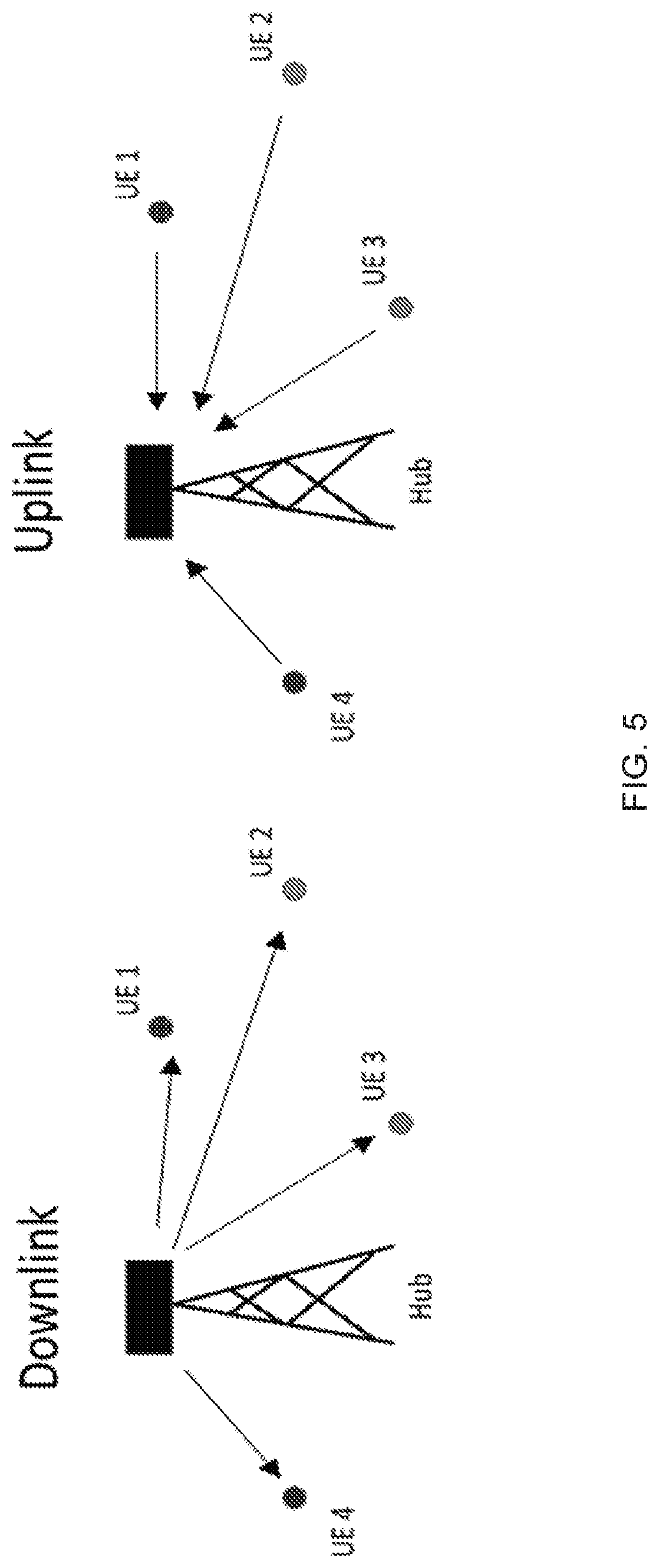
[0112] Implicit feedback is based on the principle of reciprocity which relates the uplink channel (UEs transmitting to the hub) to the downlink channel (hub transmitting to the UEs). FIG. 5 shows an example configuration of uplink and downlink channels between a hub and multiple UEs.
[0113] Specifically, denote the uplink and downlink channels by H.sub.up and H respectively, then:
H(f,t)=AH.sub.up.sup.T(f,t)B, (3)
[0114] for f=1, . . . , N.sub.f and t=1, . . . , N.sub.t. Where H.sub.up.sup.T(f,t) denotes the matrix transpose of the uplink channel. The matrices A.di-elect cons..sup.L.sup.u.sup..times.L.sup.u and B.di-elect cons..sup.L.sup.h.sup..times.L.sup.h represent hardware non-idealities. By performing a procedure called reciprocity calibration, the effect of the hardware non-idealities can be removed, thus giving a simple relationship between the uplink and downlink channels:
H(f,t)=H.sub.up.sup.T(f,t) (4)
[0115] The principle of reciprocity can be used to acquire channel knowledge at the hub. The procedure is called implicit feedback and consists of three steps.
[0116] Reciprocity calibration: the hub and UEs calibrate their hardware so that equation (4) holds.
[0117] Pilot transmission: for each time and frequency bin the UEs transmits a pilot signal denoted by p(f,t).di-elect cons..sup.L.sup.u for f=1, . . . , N.sub.f and t=1, . . . , N.sub.t. Unlike data, the pilot signal is known at both the hub and the UEs.
[0118] Channel acquisition: for each time and frequency bin the hub receives the pilot signal distorted by the uplink channel and white noise:
H.sub.up(f,t)p(f,t)+w(f,t) (5)
[0119] for f=1, . . . , N.sub.f and t=1, . . . , N.sub.t. Because the pilot signal is known by the hub, it can use signal processing to compute an estimate of the uplink channel, denoted by (f,t). Because reciprocity calibration has been performed the hub can take the transpose to get an estimate of the downlink channel, denoted by H(f,t).
[0120] The advantage of implicit feedback is that it allows the hub to acquire channel knowledge with very little overhead; the disadvantage is that reciprocity calibration is difficult to implement.
[0121] Channel Prediction
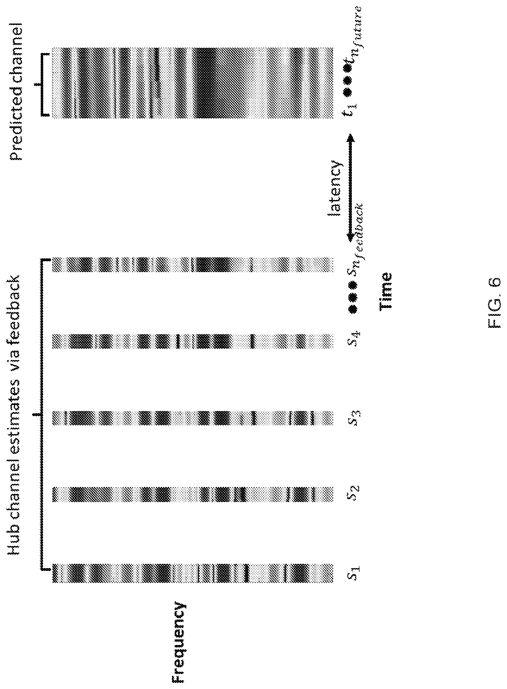
[0122] Using either explicit or implicit feedback, the hub acquires estimates of the downlink wireless channel at certain times denoted by s.sub.1,s.sub.2, . . . ,s.sub.n using these estimates it must then predict what the channel will be at future times when the precoding will be performed, denoted by t.sub.1, t.sub.2, . . . , t.sub.m. FIG. 6 shows this setup in which "snapshots" of channel are estimated, and based on the estimated snapshots, a prediction is made regarding the channel at a time in the future. As depicted in FIG. 6, channel estimates may be available across the frequency band at a fixed time slots, and based on these estimates, a predicated channel is calculated.
[0123] There are tradeoffs when choosing the feedback times s.sub.1, s.sub.2, . . . , s.sub.n.
[0124] Latency of extrapolation: Refers to the temporal distance between the last feedback time, s.sub.n, and the first prediction time, t.sub.1, determines how far into the future the hub needs to predict the channel. If the latency of extrapolation is large, then the hub has a good lead time to compute the pre-coding filters before it needs to apply them. On the other hand, larger latencies give a more difficult prediction problem.
[0125] Density: how frequent the hub receives channel measurements via feedback determines the feedback density. Greater density leads to more accurate prediction at the cost of greater overhead.
[0126] There are many channel prediction algorithms in the literature. They differ by what assumptions they make on the mathematical structure of the channel. The stronger the assumption, the greater the ability to extrapolate into the future if the assumption is true. However, if the assumption is false then the extrapolation will fail. For example:
[0127] Polynomial extrapolation: assumes the channel is smooth function. If true, can extrapolate the channel a very short time into the future .apprxeq.0.5 ms.
[0128] Bandlimited extrapolation: assumes the channel is a bandlimited function. If true, can extrapolated a short time into the future .apprxeq.1 ms.
[0129] MUSIC extrapolation: assumes the channel is a finite sum of waves. If true, can extrapolate a long time into the future .apprxeq.10 ms.
[0130] Precoding Filter Computation and Application
[0131] Using extrapolation, the hub computes an estimate of the downlink channel matrix for the times the pre-coded data will be transmitted. The estimates are then used to construct precoding filters. Precoding is performed by applying the filters on the data the hub wants the UEs to receive. Before going over details we introduce notation.
[0132] Channel estimate: for each time and frequency bin the hub has an estimate of the downlink channel which we denote by H(f,t).di-elect cons..sup.L.sup.u.sup..times.L.sup.h, for f=1, . . . , N.sub.f and t=1, . . . ,N.sub.t.
[0133] Precoding filter: for each time and frequency bin the hub uses the channel estimate to construct a precoding filter which we denote by W(f,t).di-elect cons..sup.L.sup.h.sup..times.L.sup.u for f=1, . . . , N.sub.f and t=1, . . . , N.sub.t.
[0134] Data: for each time and frequency bin the UE wants to transmit a vector of data to the UEs which we denote by x(f,t).di-elect cons..sup.L.sup.u for f=1, . . . , N.sub.f and t=1, . . . , N.sub.t.
[0135] Hub Energy Constraint
[0136] When the precoder filter is applied to data, the hub power constraint is an important consideration. We assume that the total hub transmit energy cannot exceed N.sub.fN.sub.tL.sub.h. Consider the pre-coded data:
W(f,t)x(f,t), (6)
[0137] for f=1, . . . , N.sub.f and t=1, . . . , N.sub.t. To ensure that the pre-coded data meets the hub energy constraints the hub applies normalization, transmitting:
.lamda.W(f,t)x(f,t), (7)
[0138] for f=1, . . . , N.sub.f and t=1, . . . , N.sub.t. Where the normalization constant .lamda. is given by:
.lamda. = N f N t L h f , t W ( f , t ) x ( f , t ) 2 ( 8 ) ##EQU00001##
[0139] Receiver SNR
[0140] The pre-coded data then passes through the downlink channel, the UEs receive the following signal:
.lamda.H(f,t)W(f,t)x(f,t)+w(f,t), (9)
[0141] for f=1, . . . , N.sub.f and t=1, . . . , N.sub.t. The UE then removes the normalization constant, giving a soft estimate of the data:
x soft ( f , t ) = H ( f , t ) x ( f , t ) + 1 .lamda. w ( f , t ) , ( 10 ) ##EQU00002##
[0142] for f=1, . . . , N.sub.f and t=1, . . . , N.sub.t. The error of the estimate is given by:
x soft ( f , t ) - x ( f , t ) = H ( f , t ) W ( f , t ) x ( f , t ) - x ( f , t ) + 1 .lamda. w ( f , t ) , ( 11 ) ##EQU00003##
[0143] The error of the estimate can be split into two terms. The term H(f,t)W(f,t) x(f,t) is the interference experienced by the UEs while the term
1 .lamda. w ( f , t ) ##EQU00004##
gives the noise experienced by the UEs.
[0144] When choosing a pre-coding filter there is a tradeoff between interference and noise. We now review the two most popular pre-coder filters: zero-forcing and regularized zero-forcing.
[0145] Zero Forcing Precoder
[0146] The hub constructs the zero forcing pre-coder (ZFP) by inverting its channel estimate:
w.sub.ZF(f,t)=(H*(f,t)H(f,t).sup.-1H*(f,t), (12)
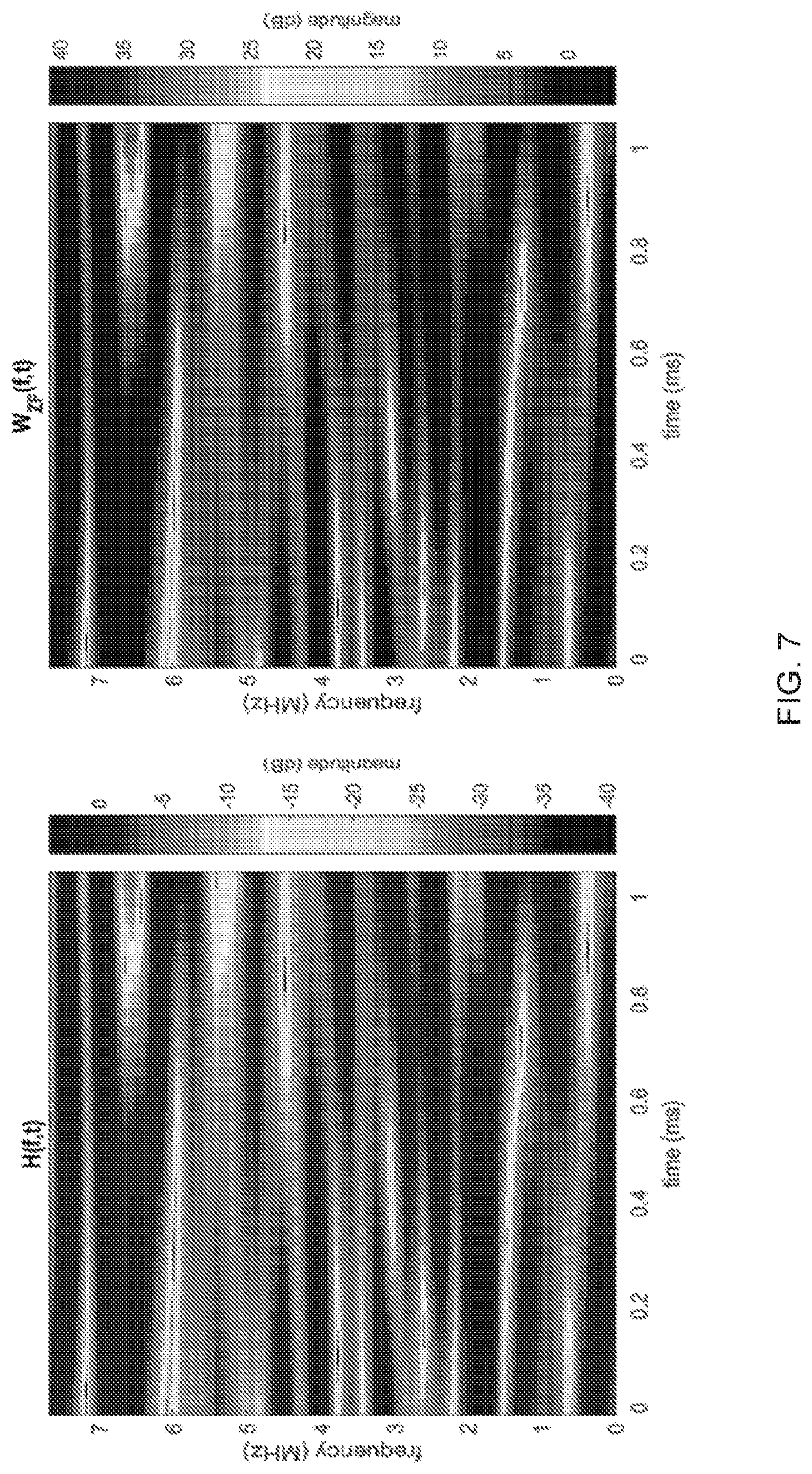
[0147] for f=1, . . . , N.sub.f and t=1, . . . , N.sub.t. The advantage of ZPP is that the UEs experience little interference (if the channel estimate is perfect then the UEs experience no interference). The disadvantage of ZFP is that the UEs can experience a large amount of noise. This is because at time and frequency bins where the channel estimate A (f,t) is very small the filter W.sub.ZF (f,t) will be very large, thus causing the normalization constant A to be very small giving large noise energy. FIG. 7 demonstrates this phenomenon for a SISO channel.
[0148] Regularized Zero-Forcing Pre-Coder (rZFP)
[0149] To mitigates the effect of channel nulls (locations where the channel has very small energy) the regularized zero forcing precoder (rZFP) is constructed be taking a regularized inverse of its channel estimate:
W.sub.rZF(f,t)=(H*(f,t)H(f,t)+.alpha.I).sup.-1H*(f,t), (13)
[0150] for f=1, . . . , N.sub.f and t=1, . . . , N.sub.t. Where .alpha.>0 is the normalization constant. The advantage of rZFP is that the noise energy is smaller compared to ZPF. This is because rZFP deploys less energy in channel nulls, thus the normalization constant .lamda. is larger giving smaller noise energy. The disadvantage of rZFP is larger interference compared to ZFP. This is because the channel is not perfectly inverted (due to the normalization constant), so the UEs will experience residual interference. FIG. 8 demonstrates this phenomenon for a SISO channel.
[0151] As described above, there are three components to a precoding system: a channel feedback component, a channel prediction component, and a pre-coding filter component. The relationship between the three components is displayed in FIG. 9.
[0152] OTFS Precoding System
[0153] Various techniques for implementing OTFS precoding system are discussed. Some disclosed techniques can be used to provide unique ability to shape the energy distribution of the transmission signal. For example, energy distribution may be such that the energy of the signal will be high in regions of time frequency and space where the channel information and the channel strength are strong. Conversely, the energy of the signal will be low in regions of time frequency and space where the channel information or the channel strength are weak.
[0154] Some embodiments may be described with reference to three main blocks, as depicted in FIG. 10.
[0155] Channel prediction: During channel prediction, second order statistics are used to build a prediction filter along with the covariance of the prediction error.
[0156] Optimal precoding filter: using knowledge of the predicted channel and the covariance of the prediction error: the hub computes the optimal precoding filter. The filter shapes the spatial energy distribution of the transmission signal.
[0157] Vector perturbation: using knowledge of the predicted channel, precoding filter, and prediction error, the hub perturbs the transmission signal. By doing this the hub shapes the time, frequency, and spatial energy distribution of the transmission signal.
[0158] Review of OTFS Modulation
[0159] A modulation is a method to transmit a collection of finite symbols (which encode data) over a fixed allocation of time and frequency. A popular method used today is Orthogonal Frequency Division Multiplexing (OFDM) which transmits each finite symbol over a narrow region of time and frequency (e.g., using subcarriers and timeslots). In contrast, Orthogonal Time Frequency Space (OTFS) transmits each finite symbol over the entire allocation of time and frequency. Before going into details, we introduce terminology and notation.
[0160] We call the allocation of time and frequency a frame. We denote the number of subcarriers in the frame by N.sub.f. We denote the subcarrier spacing by df. We denote the number of OFDM symbols in the frame by N.sub.t. We denote the OFDM symbol duration by dt. We call a collection of possible finite symbols an alphabet, denoted by A.
[0161] A signal transmitted over the frame, denoted by .phi., can be specified by the values it takes for each time and frequency bin:
.phi.(f,t).di-elect cons., (14)
[0162] for f=1, . . . , N.sub.f and t=1, . . . , N.sub.t.
[0163] FIG. 11 shows an example of a frame along time (horizontal) axis and frequency (vertical) axis. FIG. 12 shows an example of the most commonly used alphabet: Quadrature Amplitude Modulation (QAM).
[0164] OTFS Modulation
[0165] Suppose a transmitter has a collection of N.sub.fN.sub.t QAM symbols that the transmitter wants to transmit over a frame, denoted by:
x(f,t).di-elect cons.A, (15)
[0166] for f=1, . . . , N.sub.f and t=1, . . . , N.sub.t. OFDM works by transmitting each QAM symbol over a single time frequency bin:
.phi.(f,t)=x(f,t), (16)
[0167] for f=1, . . . , N.sub.f and t=1, . . . , N.sub.t. The advantage of OFDM is its inherent parallelism, this makes many computational aspects of communication very easy to implement. The disadvantage of OFDM is fading, that is, the wireless channel can be very poor for certain time frequency bins. Performing pre-coding for these bins is very difficult.
[0168] The OTFS modulation is defined using the delay Doppler domain, which is relating to the standard time frequency domain by the two-dimensional Fourier transform.
[0169] The delay dimension is dual to the frequency dimension. There are N.sub..tau. delay bins with N.sub..tau.=N.sub.f. The Doppler dimension is dual to the time dimension. There are N.sub..nu. Doppler bins with N.sub..nu.=N.sub.t.
[0170] A signal in the delay Doppler domain, denoted by .PHI., is defined by the values it takes for each delay and Doppler bin:
.PHI.(.tau.,.nu.).di-elect cons., (16)
[0171] for .tau.=1, . . . , N.sub..tau. and .nu.=1, . . . , N.sub..nu..
[0172] Given a signal .PHI. in the delay Doppler domain, some transmitter embodiments may apply the two-dimensional Fourier transform to define a signal .phi. in the time frequency domain:
.phi.(f,t)=(F.PHI.)(f,t), (17)
[0173] for f=1, . . . , N.sub.f and t=1, . . . , N.sub.t. Where F denotes the two-dimensional Fourier transform.
[0174] Conversely, given a signal .phi. in the time frequency domain, transmitter embodiments could apply the inverse two-dimensional Fourier transform to define a signal .PHI. in the delay Doppler domain:
.PHI.(.tau.,.nu.)=(F.sup.-1.phi.)(.tau.,.nu.), (18)
[0175] for .tau.=1, . . . , N.sub..tau. and .nu.=1, . . . , N.sub..nu..
[0176] FIG. 13 depicts an example of the relationship between the delay Doppler and time frequency domains.
[0177] The advantage of OTFS is that each QAM symbol is spread evenly over the entire time frequency domain (by the two-two-dimensional Fourier transform), therefore each QAM symbol experience all the good and bad regions of the channel thus eliminating fading. The disadvantage of OTFS is that the QAM spreading adds computational complexity.
[0178] MMSE Channel Prediction
[0179] Channel prediction is performed at the hub by applying an optimization criterion, e.g., the Minimal Mean Square Error (MMSE) prediction filter to the hub's channel estimates (acquired by either implicit or explicit feedback). The MMSE filter is computed in two steps. First, the hub computes empirical estimates of the channel's second order statistics. Second, using standard estimation theory, the hub uses the second order statistics to compute the MMSE prediction filter. Before going into details, we introduce notation:
[0180] We denote the number of antennas at the hub by L.sub.h. We denote the number of UE antennas by L.sub.u. We index the UE antennas by u=1, . . . , L.sub.u. We denote the number frequency bins by N.sub.f. We denote the number of feedback times by n.sub.past. We denote the number of prediction times by n.sub.future FIG. 14 shows an example of an extrapolation process setup.
[0181] For each UE antenna, the channel estimates for all the frequencies, hub antennas, and feedback times can be combined to form a single N.sub.fL.sub.hn.sub.past dimensional vector. We denote this by:
H.sub.past(u).di-elect cons..sup.N.sup.f.sup.L.sup.h.sup.n.sup.past, (19)
[0182] Likewise, the channel values for all the frequencies, hub antennas, and prediction times can be combined to form a single N.sub.fL.sub.hn.sub.future dimensional vector. We denote this by:
H.sub.future(u).di-elect cons..sup.N.sup.f.sup.L.sup.h.sup.n.sup.future, (20)
n.sub.future
[0183] In typical implementations, these are extremely high dimensional vectors and that in practice some form of compression should be used. For example, principal component compression may be one compression technique used.
[0184] Empirical Second Order Statistics
[0185] Empirical second order statistics are computed separately for each UE antenna in the following way:
[0186] At fixed times, the hub receives through feedback N samples of H.sub.past(u) and estimates of H.sub.future(u) We denote them by: H.sub.past(u).sub.i and H.sub.future(u).sub.i for i=1, . . . , N.
[0187] The hub computes an estimate of the covariance of H.sub.past(u), which we denote by {circumflex over (R)}.sub.past(u):
R ^ past ( u ) = 1 N i = 1 N H ^ past ( u ) i H ^ past ( u ) i * ( 21 ) ##EQU00005##
[0188] The hub computes an estimate of the covariance of H.sub.future (u), which we denote by {circumflex over (R)}.sub.future(u):
R ^ future ( u ) = 1 N i = 1 N H ^ future ( u ) i H ^ future ( u ) i * ( 22 ) ##EQU00006##
[0189] The hub computes an estimate of the correlation between H.sub.future (u) and H.sub.past(u), which we denote by {circumflex over (R)}.sub.past,future(u):
R ^ future , past ( u ) = 1 N i = 1 N H ^ future ( u ) i H ^ past ( u ) i * ( 23 ) ##EQU00007##
[0190] In typical wireless scenarios (pedestrian to highway speeds) the second order statistics of the channel change slowly (on the order of 1-10 seconds). Therefore, they should be recomputed relatively infrequently. Also, in some instances it may be more efficient for the UEs to compute estimates of the second order statistics and feed these back to the hub.
[0191] MMSE Prediction Filter
[0192] Using standard estimation theory, the second order statistics can be used to compute the MMSE prediction filter for each UE antenna:
C(u)=={circumflex over (R)}.sub.future,past(u){circumflex over (R)}.sub.past.sup.-1(u) (24)
[0193] Where C(u) denotes the MMSE prediction filter. The hub can now predict the channel by applying feedback channel estimates into the MMSE filter:
H.sub.future(u)=C(u)H.sub.past(u) (25)
[0194] Prediction Error Variance
[0195] We denote the MMSE prediction error by .DELTA.H.sub.future(u), then:
H.sub.future(u)=H.sub.future(u)+.DELTA.H.sub.future(u). (26)
[0196] We denote the covariance of the MMSE prediction error by R.sub.error(u), with:
R.sub.error(u)=[.DELTA.H.sub.future(u).DELTA.H.sub.future(u)*] (27)
[0197] Using standard estimation theory, the empirical second order statistics can be used to compute an estimate of R.sub.error(u):
{circumflex over (R)}.sub.error(u)=C(U){circumflex over (R)}.sub.past(u)C(u)*-C(u){circumflex over (R)}.sub.future,past(u)*-{circumflex over (R)}.sub.future,past(u)C(u)*+{circumflex over (R)}.sub.future(u) (28)
[0198] Simulation Results
[0199] We now present simulation results illustrating the use of the MMSE filter for channel prediction. Table 1 gives the simulation parameters and FIG. 15 shows the extrapolation setup for this example.
TABLE-US-00001 TABLE 1 Subcarrier spacing 15 kHz Number of subcarriers 512 Delay spread 3 .mu.s Doppler spread 600 Hz Number of channel 5 feedback estimates Spacing of channel 10 ms feedback estimates Prediction range 0-20 ms into the future
[0200] Fifty samples of H.sub.past and H.sub.future were used to compute empirical estimates of the second order statistics. The second order statistics were used to compute the MMSE prediction filter. FIG. 16 shows the results of applying the filter. The results have shown that the prediction is excellent at predicting the channel, even 20 ms into the future.
[0201] Block Diagrams
[0202] In some embodiments, the prediction is performed independently for each UE antenna. The prediction can be separated into two steps:
[0203] 1) Computation of the MMSE prediction filter and prediction error covariance: the computation can be performed infrequently (on the order of seconds). The computation is summarized in FIG. 17. Starting from left in FIG. 17, first, feedback channel estimates are collected. Next, the past, future and future/past correlation matrices are computed. Next the filter estimate C(u) and the error estimate are computed.
[0204] 2) Channel prediction: is performed every time pre-coding is performed. The procedure is summarized in FIG. 18.
[0205] Optimal Precoding Filter
[0206] Using MMSE prediction, the hub computes an estimate of the downlink channel matrix for the allocation of time and frequency the pre-coded data will be transmitted. The estimates are then used to construct precoding filters. Precoding is performed by applying the filters on the data the hub wants the UEs to receive. Embodiments may derive the "optimal" precoding filters as follows. Before going over details we introduce notation.
[0207] Frame (as defined previously): precoding is performed on a fixed allocation of time and frequency, with N.sub.f frequency bins and N.sub.t time bins. We index the frequency bins by: f=1, . . . , N.sub.f. We index the time bins by t=1, . . . ,N.sub.t.
[0208] Channel estimate: for each time and frequency bin the hub has an estimate of the downlink channel which we denote by H(f,t).di-elect cons..sup.L.sup.u.sup..times.L.sup.h.
[0209] Error correlation: we denote the error of the channel estimates by .DELTA.H(f,t), then:
H(f,t)=H(f,t)+.DELTA.H(f,t), (29)
[0210] We denote the expected matrix correlation of the estimation error by R.sub..DELTA.H(f,t).di-elect cons..sup.L.sup.h.sup..times.L.sup.h, with:
R.sub..DELTA.H(f,t)=[.DELTA.H(f,t)*.DELTA.H(f,t)]. (30)
[0211] The hub can be easily compute these using the prediction error covariance matrices computed previously: {circumflex over (R)}.sub.error(U) for u=1, . . . , L.sub.u.
[0212] Signal: for each time and frequency bin the UE wants to transmit a signal to the UEs which we denote by s(f,t).di-elect cons..sup.L.sup.u.
[0213] Precoding filter: for each time and frequency bin the hub uses the channel estimate to construct a precoding filter which we denote by W(f,t).di-elect cons..sup.L.sup.h.sup..times.L.sup.u.
[0214] White noise: for each time and frequency bin the UEs experience white noise which we denote by n(f,t).di-elect cons..sup.L.sup.u. We assume the white noise is iid Gaussian with mean zero and variance N.sub.0.
[0215] Hub Energy Constraint
[0216] When the precoder filter is applied to data, the hub power constraint may be considered. We assume that the total hub transmit energy cannot exceed N.sub.fN.sub.tL.sub.h. Consider the pre-coded data:
W(f,t)s(f,t), (31)
[0217] To ensure that the pre-coded data meets the hub energy constraints the hub applies normalization, transmitting:
.lamda.W(f,t)s(f,t), (32)
[0218] Where the normalization constant .lamda. is given by:
.lamda. = N f N t L h f , t W ( f , t ) s ( f , t ) 2 ( 33 ) ##EQU00008##
[0219] Receiver SINR
[0220] The pre-coded data then passes through the downlink channel, the UEs receive the following signal:
.lamda.H(f,t)W(f,t)s(f,t)+n(f,t), (34)
[0221] The UEs then removes the normalization constant, giving a soft estimate of the signal:
s soft ( f , t ) = H ( f , t ) W ( f , t ) s ( f , t ) + 1 .lamda. n ( f , t ) . ( 35 ) ##EQU00009##
[0222] The error of the estimate is given by:
s soft ( f , t ) - s ( f , t ) = H ( f , t ) W ( f , t ) s ( f , t ) - s ( f , t ) + 1 .lamda. n ( f , t ) . ( 36 ) ##EQU00010##
[0223] The error can be decomposed into two independent terms: interference and noise. Embodiments can compute the total expected error energy:
expected error energy = f = 1 N f t = 1 N t s soft ( f , t ) - s ( f , t ) 2 = f = 1 N f t = 1 N t H ( f , t ) W ( f , t ) s ( f , t ) - s ( f , t ) 2 + 1 .lamda. 2 n ( f , t ) 2 = f = 1 N f t = 1 N t ( H ^ ( f , t ) W ( f , t ) s ( f , t ) - s ( f , t ) ) * ( H ^ ( f , t ) W ( f , t ) s ( f , t ) - s ( f , t ) ) + ( W ( f , t ) s ( f , t ) ) * ( R .DELTA. H ( f , t ) + N 0 L u L h I ) ( W ( f , t ) s ( f , t ) ) ( 37 ) ##EQU00011##
[0224] Optimal Precoding Filter
[0225] We note that the expected error energy is convex and quadratic with respect to the coefficients of the precoding filter. Therefore, calculus can be used to derive the optimal precoding filter:
W opt ( f , t ) = ( H ^ ( f , t ) * H ^ ( f , t ) + R .DELTA. H ( f , t ) + N 0 L u L h I ) - 1 H ^ ( f , t ) * ( 38 ) ##EQU00012##
[0226] Accordingly, some embodiments of an OTFS precoding system use this filter (or an estimate thereof) for precoding.
[0227] Simulation Results
[0228] We now present a simulation result illustrating the use of the optimal precoding filter. The simulation scenario was a hub transmitting data to a single UE. The channel was non line of sight, with two reflector clusters: one cluster consisted of static reflectors, the other cluster consisted of moving reflectors. FIG. 19 illustrates the channel geometry, with horizontal and vertical axis in units of distance. It is assumed that the hub has good Channel Side Information (CSI) regarding the static cluster and poor CSI regarding the dynamic cluster. The optimal precoding filter was compared to the MMSE precoding filter. FIG. 20 displays the antenna pattern given by the MMSE precoding filter. It can be seen that the energy is concentrated at .+-.45.degree., that is, towards the two clusters. The UE SINR is 15.9 dB, the SINR is relatively low due to the hub's poor CSI for the dynamic cluster.
[0229] FIG. 21 displays the antenna pattern given by the optimal precoding filter as described above, e.g., using equation (38). In this example, the energy is concentrated at 45.degree., that is, toward the static cluster. The UE SINR is 45.3 dB, the SINR is high (compared to the MMSE case) due to the hub having good CSI for the static reflector.
[0230] The simulation results depicted in FIG. 20 and FIG. 21 illustrate the advantage of the optimal pre-coding filter. The filter it is able to avoid sending energy towards spatial regions of poor channel CSI, e.g., moving regions.
[0231] Example Block Diagrams
[0232] Precoding is performed independently for each time frequency bin. The precoding can be separated into three steps:
[0233] [1] Computation of error correlation: the computation be performed infrequently (on the order of seconds). The computation is summarized in FIG. 22.
[0234] [2] Computation of optimal precoding filter: may be performed every time pre-coding is performed. The computation is summarized in FIG. 23.
[0235] [3] Application of the optimal precoding filter: may be performed every time pre-coding is performed. The procedure is summarized in FIG. 24.
[0236] OTFS Vector Perturbation
[0237] Before introducing the concept of vector perturbation, we outline the application of the optimal pre-coding filter to OTFS.
[0238] OTFS Optimal Precoding
[0239] In OTFS, the data to be transmitted to the UEs are encoded using QAMs in the delay-Doppler domain. We denote this QAM signal by x, then:
x(.tau.,.nu.).di-elect cons.A.sup.L.sup.u, (39)
[0240] for .tau.=1, . . . , N.sub..tau. and .nu.=1, . . . , N.sub..nu.. A denotes the QAM constellation. Using the two-dimensional Fourier transform the signal can be represented in the time frequency domain. We denote this representation by X:
X(f,t)=(Fx)(f,t), (40)
[0241] for f=1, . . . , N.sub.f and t=1, . . . , N.sub.t. F denotes the two-dimensional Fourier transform. The hub applies the optimal pre-coding filter to X and transmit the filter output over the air:
.lamda.W.sub.opt(f,t)X(f,t), (41)
[0242] for f=1, . . . , N.sub.f and t=1, . . . , N.sub.t. .lamda. denotes the normalization constant. The UEs remove the normalization constant giving a soft estimate of X:
X soft ( f , t ) = H ( f , t ) W opt ( f , t ) X ( f , t ) + 1 .lamda. w ( f , t ) , ( 42 ) ##EQU00013##
[0243] for f=1, . . . , N.sub.f and t=1, . . . , N.sub.t. The term w(f,t) denotes white noise. We denote the error of the soft estimate by E:
E(f,t)=X.sub.soft(f,t)-X(f,t), (43)
[0244] for f=1, . . . , N.sub.f and t=1, . . . , N.sub.t. The expected error energy was derived earlier in this document:
expected error energy = f = 1 N f t = 1 N t X soft ( f , t ) - X ( f , t ) 2 = f = 1 N f t = 1 N t X ( f , t ) * M error ( f , t ) X ( f , t ) ( 44 ) ##EQU00014##
[0245] Where:
M error ( f , t ) = ( H ^ ( f , t ) W opt ( f , t ) - 1 ) * ( H ^ ( f , t ) W opt ( f , t ) - I ) + W opt ( f , t ) * ( R .DELTA. H ( f , t ) + N 0 L u L h ) W opt ( f , t ) ( 45 ) ##EQU00015##
[0246] We call the positive definite matrix M.sub.error(f,t) the error metric.
[0247] Vector Perturbation
[0248] In vector perturbation, the hub transmits a perturbed version of the QAM signal:
x(.tau.,.nu.)+p(.tau.,.nu.), (46)
[0249] for .tau.=1, . . . , N.sub..tau. and .nu.=1, . . . , N.sub..nu.. Here, p(.tau.,.nu.) denotes the perturbation signal. The perturbed QAMs can be represented in the time frequency domain:
X(f,t)+P(f,t)=(Fx)(f,t)+(Fp)(f,t), (47)
[0250] for f=1, . . . , N.sub.f and t=1, . . . , N.sub.t. The hub applies the optimal pre-coding filter to the perturbed signal and transmits the result over the air. The UEs remove the normalization constant giving a soft estimate of the perturbed signal:
X(f,t)+P(f,t)+E(f,t), (48)
[0251] for f=1, . . . , N.sub.f and t=1, . . . , N.sub.t. Where E denotes the error of the soft estimate. The expected energy of the error is given by:
expected error energy=.SIGMA..sub.f=1.sup.N.sup.f.SIGMA..sub.t=1.sup.N.sup.t(X(f,t)+P(f,- t))*M.sub.error(f,t)(X(f,t)+P(f,t)) (49)
[0252] The UEs then apply an inverse two dimensional Fourier transform to convert the soft estimate to the delay Doppler domain:
x(.tau.,.nu.)+p(.tau.,.nu.)+e(.tau.,.nu.), (50)
[0253] for .tau.=1, . . . , N.sub..tau. and .nu.=1, . . . , N.sub..nu.. The UEs then remove the perturbation p(.tau.,.nu.) for each delay Doppler bin to recover the QAM signal x.
[0254] Collection of Vector Perturbation Signals
[0255] One question is: what collection of perturbation signals should be allowed? When making this decision, there are two conflicting criteria:
[0256] 1) The collection of perturbation signals should be large so that the expected error energy can be greatly reduced.
[0257] 2) The collection of perturbation signals should be small so the UE can easily remove them (reduced computational complexity):
x(.tau.,.nu.)+p(.tau.,.nu.).fwdarw.x(.tau.,.nu.) (51)
[0258] Coarse Lattice Perturbation
[0259] An effective family of perturbation signals in the delay-Doppler domain, which take values in a coarse lattice:
p(.tau.,.nu.).di-elect cons.B.sup.L.sup.u, (52)
[0260] for .tau.=1, . . . , N.sub..tau. and .nu.=1, . . . , N.sub..nu.. Here, B denotes the coarse lattice. Specifically, if the QAM symbols lie in the box: [-r,r].times.j[-r,r] we take as our perturbation lattice B=2r+2rj. We now illustrate coarse lattice perturbation with an example.
EXAMPLES
[0261] Consider QPSK (or 4-QAM) symbols in the box [-2,2].times.j[-2,2]. The perturbation lattice is then B=4+4j. FIG. 25 illustrates the symbols and the lattice. Suppose the hub wants to transmit the QPSK symbol 1+1j to a UE. Then there is an infinite number of coarse perturbations of 1+1j that the hub can transmit. FIG. 26 illustrates an example. The hub selects one of the possible perturbations and transmits it over the air. FIG. 27 illustrates the chosen perturbed symbol, depicted with a single solid circle.
[0262] The UE receives the perturbed QPSK symbol. The UE then removes the perturbation to recover the QPSK symbol. To do this, the UE first searches for the coarse lattice point closest to the received signal. FIG. 28 illustrates this.
[0263] The UE subtracts the closest lattice point from the received signal, thus recovering the QPSK symbol 1+1j. FIG. 29 illustrates this process.
[0264] Finding Optimal Coarse Lattice Perturbation Signal
[0265] The optimal coarse lattice perturbation signal, p.sub.opt, is the one which minimizes the expected error energy:
p.sub.opt=arg min.sub.p.SIGMA..sub.f=1.sup.N.sup.f.SIGMA..sub.t=1.sup.N.sup.t(X(f,t)+P(- f,t))*M.sub.error(f,t)(X(f,t)+P(f,t)) (53)
[0266] The optimal coarse lattice perturbation signal can be computed using different methods. A computationally efficient method is a form of Thomlinson-Harashima precoding which involves applying a DFE filter at the hub.
[0267] Coarse Lattice Perturbation Example
[0268] We now present a simulation result illustrating the use of coarse lattice perturbation. The simulation scenerio was a hub antenna transmitting to a single UE antenna. Table 2 displays the modulation paramaters. Table 3 display the channel paramaters for this example.
TABLE-US-00002 TABLE 2 Subcarrier spacing 30 kHz Number of 256 subcarriers OFDM symbols 32 per frame QAM order Infinity (uniform in the unit box)
TABLE-US-00003 TABLE 3 Number of reflectors 20 Delay spread 2 .mu.s Doppler spread 1 KHz Noise variance -35 dB
[0269] FIG. 30 displays the channel energy in the time (horizontal axis) and frequency (vertical axis) domain.
[0270] Because this is a SISO (single input single output) channel, the error metric M.sub.error (f,t) is a positive scaler for each time frequency bin. The expected error energy is given by integrating the product of the error metric with the perturbed signal energy:
expected error energy=.SIGMA..sub.f=1.sup.N.sup.f.SIGMA..sub.t=1.sup.N.sup.tM.sub.error(- f,t)|X(f,t)+P(f,t)|.sup.2 (54)
[0271] FIG. 31 displays an example of the error metric. One hundred thousand random QAM signals were generated. For each QAM signal, the corresponding optimal perturbation signal was computed using Thomlinson-Harashima precoding. FIG. 32 compares the average energy of the QAM signals with the average energy of the perturbed QAM signals. The energy of QAM signals is white (evenly distributed) while the energy of the perturbed QAM signals is colored (strong in some time frequency regions and weak in others). The average error energy of the unperturbed QAM signal was -24.8 dB. The average error energy of the perturbed QAM signal was -30.3 dB. The improvement in error energy can be explained by comparing the energy distribution of the perturbed QAM signal with the error metric.
[0272] FIG. 33 shows a comparison of an example error metric with an average perturbed QAM energy. The perturbed QAM signal has high energy where the error metric is low, conversely it has low energy where the error metric is high.
[0273] The simulation illustrates the gain from using vector perturbation: shaping the energy of the signal to avoid time frequency regions where the error metric is high.
[0274] Block Diagrams
[0275] Vector perturbations may be performed in three steps. First, the hub perturbs the QAM signal. Next, the perturbed signal is transmitted over the air using the pre-coding filters. Finally, the UEs remove the perturbation to recover the data.
[0276] Computation of error metric: the computation can be performed independently for each time frequency bin. The computation is summarized in FIG. 34. See also Eq. (45). As shown, the error metric is calculated using channel prediction estimate, the optimal coding filter and error correlation estimate.
[0277] Computation of perturbation: the perturbation is performed on the entire delay Doppler signal. The computation is summarized in FIG. 35. As shown, the QAM signal and the error metric are used to compute the perturbation signal. The calculated perturbation signal is additively applied to the QAM input signal.
[0278] Application of the optimal precoding filter: the computation can be performed independently for each time frequency bin. The computation is summarized in FIG. 36. The perturbed QAM signal is processed through a two dimensional Fourier transform to generate a 2D transformed perturbed signal. The optimal precoding filter is applied to the 2D transformed perturbed signal.
[0279] UEs removes perturbation: the computation can be FIG. 37. At UE, the input signal received is transformed through an inverse 2D Fourier transform. The closest lattice point for the resulting transformed signal is determined and then removed from the 2D transformed perturbed signal.
[0280] Spatial Tomlinson Harashima Precoding
[0281] This section provides additional details of achieving spatial precoding and the beneficial aspects of using Tomlinson Harashima precoding algorithm in implementing spatial precoding in the delay Doppler domain. The embodiments consider a flat channel (with no frequency or time selectivity).
[0282] Review of Linear Precoding
In precoding, the hub wants to transmit a vector of QAMs to the UEs. We denote this vector by x.di-elect cons..sup.L.sup.u. The hub has access to the following information: [0283] An estimate of the downlink channel, denoted by: H.di-elect cons..sup.L.sup.u.sup..times.L.sup.h. [0284] The matrix covariance of the channel estimation error, denoted by: R.sub..DELTA.H.di-elect cons..sup.L.sup.h.sup..times.L.sup.h. From this information, the hub computes the "optimal" precoding filter, which minimizes the expected error energy experienced by the UEs:
[0284] W opt = ( H ^ * H ^ + R .DELTA. H + N 0 L u L h I ) - 1 H ^ * ##EQU00016##
By applying the precoding filter to the QAM vector the hub constructs a signal to transmit over the air: .lamda.W.sub.opt.times..di-elect cons..sup.L.sup.h, where .lamda. is a constant used to enforce the transmit energy constraints. The signal passes through the downlink channel and is received by the UEs:
.lamda.HW.sub.optx+w,
Where w.di-elect cons..sup.L.sup.u denotes AWGN noise. The UEs remove the normalization constant giving a soft estimate of the QAM signal:
x+e,
where e.di-elect cons..sup.L.sup.u denotes the estimate error. The expected error energy can be computed using the error metric:
expected error energy=x*M.sub.errorx
where M.sub.error is a positive definite matrix computed by:
M error = ( H ^ W opt - I ) * ( H ^ W opt - I ) + W opt * ( R .DELTA. H + N 0 L u L h ) W opt ##EQU00017##
[0285] Review of Vector Perturbation
The expected error energy can be greatly reduced by perturbing the QAM signal by a vector .nu..di-elect cons..sup.L.sup.u. The hub now transmits .lamda.W.sub.opt(x+.nu.).di-elect cons..sup.L.sup.h. After removing the normalization constant, the UEs have a soft estimate of the perturbed QAM signal:
x+.nu.+e
Again, the expected error energy can be computed using the error metric:
expected error energy=(x+.nu.)*M.sub.error(x+.nu.)
The optimal perturbation vector minimizes the expected error energy:
.nu..sub.opt=arg min.sub..nu.(x+.nu.)*M.sub.error(x+.nu.).
Computing the optimal perturbation vector is in general NP-hard, therefore, in practice an approximation of the optimal perturbation is computed instead. For the remainder of the document we assume the following signal and perturbation structure:
[0286] The QAMs lie in the box [-1, 1].times.j[-1, 1].
[0287] The perturbation vectors lie on the coarse lattice: (2+2j).sup.L.sup.u.
[0288] Spatial Tomlinson Harashima Precoding
In spatial THP a filter is used to compute a "good" perturbation vector. To this end, we make use of the Cholesky decomposition of the positive definite matrix M.sub.error:
M.sub.error=U*DU,
where D is a diagonal matrix with positive entries and U is unit upper triangular. Using this decomposition, the expected error energy can be expressed as:
expected error energy=(U(x+.nu.))*D(U(x+.nu.))=z*Dz=.SIGMA..sub.n=1.sup.L.sup.uD(n,n)|z(- n)|.sup.2,
where z=U(x+.nu.). We note that minimizing the expected error energy is equivalent to minimizing the energy of the z entries, where:
z ( L u ) = x ( L u ) + v ( L u ) , z ( n ) = x ( n ) + v ( n ) + m = n + 1 L u U ( n , m ) ( x ( m ) + v ( m ) ) , ##EQU00018##
for n=1, 2, . . . , L.sub.u-1. Spatial THP iteratively chooses a perturbation vector in the following way.
.nu.(L.sub.u)=0
[0289] Suppose .nu.(n+1), .nu.(n+2), . . . , .nu.(L.sub.u) have been chosen, then:
v ( n ) = - ( 2 + 2 j ) ( x ( n ) + m = n + 1 L u U ( n , m ) ( x ( m ) + v ( m ) ) ) ##EQU00019##
[0290] where .sub.(2.sub.+2j.sub.) denotes projection onto the coarse lattice. We note that by construction the coarse perturbation vector bounds the energy of the entries of z by two. FIG. 38 displays a block diagram of spatial THP.
[0291] Simulation Results
[0292] We now present the results of a simple simulation to illustrate the use of spatial THP. Table 4 summarizes the simulation setup.
TABLE-US-00004 TABLE 4 Simulation setup Number of hub 2 antennas Number of UEs 2 (one antenna each) Channel condition 10 dB number Modulation PAM infinity (data uniformly disturbed on the interval [-1, 1]) Data noise variance -35 dB Channel noise variance -35 dB
[0293] FIG. 39 displays the expected error energy for different PAM vectors. We note two aspects of the figure. [0294] The error energy is low when the signal transmitted to UE1 and UE2 are similar.
[0295] Conversely, the error energy is high when the signals transmitted to the UEs are dissimilar. We can expect this pattern to appear when two UEs are spatially close together; in these situations, it is advantageous to transmit the same message to both UEs. [0296] The error energy has the shape of an ellipses. The axes of the ellipse are defined by the eigenvectors of M.sub.error.
[0297] A large number data of PAM vectors was generated and spatial THP was applied. FIG. 40 shows the result. Note that the perturbed PAM vectors are clustered along the axis with low expected error energy.
[0298] THP Enhancements
The problem of finding the optimal perturbation vector at the transmitter is analogous to the MIMO QAM detection problem at the receiver. Furthermore, transmitter THP is analogous to receiver successive interference cancellation (SIC). The same improvements used for SIC can be used for THP, for example: [0299] V-Blast, can be used to first choose a better ordering of streams before applying THP. [0300] K-best and sphere detection can be used to search more perturbation vectors. [0301] Lattice reduction can be used as a pre-processing step to THP, improving the condition number of the Cholesky factors.
[0302] All these techniques are well known to wireless engineers. We will only go into more depth with lattice reduction as it gives the best performance for polynomial complexity.
[0303] Lattice Reduction Enhancement
The performance of THP depends strongly on the size of the diagonal Cholesky factor of M.sub.error:
expected error energy = n = 1 L u D ( n , n ) z ( n ) 2 .ltoreq. 2 n = 1 L u D ( n , n ) ##EQU00020##
Lattice reduction is a pre-processing step to THP which improves performance by relating the old Cholesky factorization U*DU to a new Cholesky factorization U*.sub.LRD.sub.LRU.sub.LR, with:
n = 1 L u D L R ( n , n ) .ltoreq. n = 1 L u D ( n , n ) ##EQU00021## D 1 2 U = AD LR 1 2 U L R T ##EQU00021.2##
[0304] where A.di-elect cons..sup.L.sup.u.sup..times.L.sup.u is a unitary matrix (i.e AA*=A*A=1), and T.di-elect cons.(+j).sup.L.sup.u.sup..times.L.sup.u is unimodular (i.e. complex integer entries with determinate 1 or -1). We note that if M.sub.error is ill-conditioned, then the diagonal of the lattice reduced Cholesky factor is typically much smaller then the original. To use the improved Cholesky factorization for THP we need to make use of two important properties of unimodular matrices:
[0305] If T is unimodular, then T.sup.-1 is also unimodular.
[0306] If .nu..SIGMA.(Z+j).sup.L.sup.u, then T.nu..di-elect cons.(+j).sup.L.sup.u.
We now return to the perturbation problem, where we are trying to find a coarse perturbation vector .nu..di-elect cons.(2L+2j).sup.L.sup.u which minimizes the expected error energy:
min v ( x + v ) * U * D U ( x + v ) = min v ( x + v ) * ( D 1 2 U ) * ( D 1 2 U ) ( x + v ) = min v ( x + v ) * ( A D LR 1 2 U L R T ) * A D LR 1 2 U L R T ( x + v ) = min v ( Tx + Tv ) * U L R * D L R U L R ( T x + T v ) = min v ~ ( Tx + v .about. ) * U L R * D L R U L R ( Tx + v .about. ) ##EQU00022##
where the last equality follows from the fact that applying unimodular matrices to coarse perturbation vectors returns coarse perturbation vectors. THP can now be used to find a coarse perturbation vector {tilde over (.nu.)} which makes (Tx+{tilde over (.nu.)})))*U*.sub.LRD.sub.LRU.sub.LR(Tx+{tilde over (.nu.)}) small. Applying T.sup.-1 to {tilde over (.nu.)} returns a coarse perturbation vector .nu. which makes (x+.nu.)*U*DU(x+.nu.) small. We now summarize the steps: 1. Compute a lattice reduced Cholesky factorization U*.sub.LRD.sub.LRU.sub.LR(The most popular algorithm for this is LAmstra-Lenstra-LovAsz basis reduction). The algorithm will return the reduced Cholesky factorization and the unimodular matrix T. 2. Use THP to find a coarse perturbation vector {tilde over (.nu.)} which makes the equation (1.) small: (Tx+{tilde over (.nu.)})*U*.sub.LRD.sub.LRU.sub.LR(Tx+{tilde over (.nu.)})(1.)
3. Return T.sup.-1{tilde over (.nu.)}.
[0307] OTFS Tomlinson Harashima Precoding Filters
[0308] This section details of techniques of efficiently computing coarse OTFS perturbation using a THP filter in the OTFS domain.
[0309] Review of OTFS Perturbation
The goal of OTFS perturbation is to find a coarse perturbation signal which makes the expected error energy small, where:
expected error energy = f = 0 N f - 1 t = 0 N t - 1 ( X ( f , t ) + P ( f , t ) ) * M error ( f , t ) ( X ( f , t ) + P ( f , t ) ) ##EQU00023##
[0310] Recall that X=.sub.TFx and P=.sub.TFp, where .sub.TF denotes the two-dimensional Fourier transform, x is the QAM signal, and p is the perturbation signal. The presence of the Fourier transform means that perturbing a single QAM in the delay-Doppler domain affects the signal over the entire time-frequency domain (illustrated in FIG. 41).
The time-frequency (TF) non-locality of OTFS perturbations carries advantages and disadvantages. [0311] Advantage: OTFS perturbations can shape the TF spectrum of the signal to avoid TF channel fades. [0312] Disadvantage: the OTFS perturbations are typically computed jointly, this contrasts with OFDM which can compute independent perturbations for each TF bin.
[0313] When OTFS perturbations are computed jointly, this means that brute force methods may not work efficiently. For example, consider the system parameters summarized in Table 5.
TABLE-US-00005 TABLE 5 Typical system parameters N.sub.f 600 N.sub..tau. 14 L.sub.u 4
[0314] For such a system the space of coarse perturbation signals, (2+2j).sup.L.sup.u.sup.N.sup.f.sup.N.sup.t, is 3.36e4 dimensional.
[0315] OTFS THP Filters
[0316] To manage the complexity of OTFS perturbations it may be recalled that the channel is localized in the delay-Doppler domain. Utilizing this fact, a near optimal coarse perturbation can be computed using a two-dimensional filter whose length is roughly equal to the delay and Doppler span of the channel. We call this class of filters OTFS THP filters. These filters can get quite sophisticated, so the document will develop them in stages: starting with simple cases and ending in full generality. [0317] 1) SISO single carrier (this is equivalent to OTFS with N.sub.t=1) [0318] 2) SISO OTFS [0319] 3) MIMO single carrier [0320] 4) MIMO OTFS
[0321] SISO Single Carrier
In this section, we disclose a SISO single carrier THP filter. Towards this end we express the expected error energy in the delay domain (the domain where QAMs and perturbations are defined):
expected error energy = f = 0 N f - 1 ( X ( f ) + P ( f ) ) * M error ( f ) ( X ( f ) + P ( f ) ) = .tau. = 0 N .tau. - 1 ( x ( .tau. ) + p ( .tau. ) ) * .tau. ' = 0 N .tau. - 1 m error ( .tau. - .tau. ' ) ( x ( .tau. ' ) + p ( .tau. ' ) ) ##EQU00024##
The QAM signal x and the perturbation signal p can be represented as vectors in .sup.N.sup..tau. which we denote by x, p respectively. Likewise, convolution by m.sub.error can be represented as multiplication by a positive definite circulant matrix in .sup.N.sup..tau..sup..times.N.sup..tau. which we denote by m.sub.error. Using these representations, we can write the expected error energy as:
expected error energy=(x+p)*m.sub.error(x+p)
[0322] Similar to the spatial case, a good coarse perturbation vector can be computed (FIG. 42) by utilizing the Cholesky factors of m.sub.error:
m.sub.error=UDU*
Although the method computes good perturbations, there are two main challenges: it requires a very large Cholesky factorization and the application of U-I can be very expensive. To resolve these issues, we will utilize U.sup.-1 which has much better structure: [0323] U.sup.-1 is bandlimited, with bandwidth approximately equal to the channel delay span. [0324] Apart from its edges, U.sup.-1 is nearly Toeplitz.
[0325] These facts enable the computation of good perturbations using a short filter which we call the SISO single carrier THP filter and denote by W.sub.THP. Before showing how to compute coarse perturbations with U.sup.-1 and W.sub.THP, we illustrate the structure of U.sup.-1 with a small simulation (parameters in Table 6).
TABLE-US-00006 TABLE 6 Sample rate 10 MHz Number of 512 samples Delay span 3 us Shaping filter Root raised cosine, roll-off 12% Data noise -35 dB variance Channel noise -35 dB variance
[0326] FIG. 43 displays an estimate of the channel impulse response. Using this estimate, the error metric in the delay domain, m.sub.error, was computed. FIG. 44 compares the structure of the resulting Cholesky factor and its inverse.
[0327] To visualize the near Toeplitz structure of U.sup.-1 we overlay plots of columns slices (FIG. 45):
s.sub.n(m)=U.sup.-1(n-m,n)
[0328] for m=0, 1, . . . , 40 and n=40, . . . , (N.sub.f-40). We note that if a matrix is Toeplitz then the slices will be identical.
[0329] FIG. 45 shows the bandwidth of U.sup.-1 is approximately equal to the channel span, and that outside of edges the matrix is very near Toeplitz.
[0330] Computing Good Perturbations with U.sup.-1
In this subsection, we disclose how to compute good perturbations using U.sup.-1. Towards this end we express the expected error energy in terms of the Cholesky factors:
expected error energy = ( x + p ) * m e r r o r ( x + p ) = ( U ( x + p ) ) * D ( U ( x + p ) ) = z * Dz = .tau. = 0 N .tau. - 1 D ( .tau. ) z ( .tau. ) 2 ##EQU00025##
where z=U (x+p) and D (.tau.)=D.sub.(.tau.,.tau.). Therefore, minimizing the expected error energy is equivalent to minimizing the energy of the entries of z, which can be expressed recursively:
z ( .tau. ) = x ( .tau. ) + p ( .tau. ) - .tau. ' = .tau. + 1 N .tau. - 1 U - 1 ( .tau. , .tau. ' ) z ( .tau. ' ) ##EQU00026##
for .tau.=0,1, . . . , N.sub..tau.-1. Using this expression, a good perturbation vector can be computed iteratively in the following way: [0331] 1. Initialization set p(N.sub..tau.-1)=0 and z(N.sub..tau.-1)=x(N.sub..tau.-1). [0332] 2. Update suppose we have selected p(.tau.') and z(.tau.') for .tau.'=(.tau.+1), . . . , N.sub.T-1, then:
[0332] r ( .tau. ) = x ( .tau. ) - .tau. ' = .tau. + 1 N .tau. - 1 U - 1 ( .tau. , .tau. ' ) z ( .tau. ' ) ##EQU00027## p ( .tau. ) = - ( 2 + 2 j ) ( r ( .tau. ) ) ##EQU00027.2## z ( .tau. ) = x ( .tau. ) + r ( .tau. ) ##EQU00027.3##
[0333] Herein, .sub.(2.sub.+2j.sub.) denotes projection onto the coarse lattice. We note that the algorithm bounds the energy of the z entries by two. FIG. 46 displays a block diagram of the algorithm.
[0334] Computing Perturbations with W.sub.THP
In this subsection, we disclose how to efficiently compute a good perturbation using a SISO single carrier THP filter. Towards this end we note that due to the banded near Toeplitz structure of U.sup.-1, the application of I-U.sup.-1 can be well approximated by the application of a filter (outside of edge effects):
.tau. ' = .tau. + 1 N .tau. - 1 U - 1 ( .tau. , .tau. ' ) z ( .tau. ' ) .apprxeq. n = 1 N chan W THP ( n ) z ( .tau. + n ) , ##EQU00028##
for .tau.=0, 1, . . . , N.sub..tau.-N.sub.chan-1, where N.sub.chan denotes the channel width. We call W.sub.THP the SISO single carrier THP filter with:
W.sub.THP(n)=U.sup.-1(N.sub.chan-n,N.sub.chan),
for n=1, . . . , N.sub.chan To use the approximation, we need to avoid the non-Toeplitz edge effects of U.sup.-1, this is done by enforcing the QAM signal x to take the value zero for an initialization region. Putting everything together gives an efficient method for computing good perturbation signals:
[0335] Setup compute the filter coefficients: W.sub.THP(n) for n=1, . . . , N.sub.chan.
[0336] Initialization set function values on the top delay bins equal to zero:
p(.tau.)=0,x(.tau.)=0, and z(.tau.)=0 [0337] for T=N.sub.T N.sub.chan, . . . , N.sub..tau.-1
[0338] Update suppose we have selected p(.tau.') and z(.tau.') for .tau.'=(.tau.+1), . . . , N.sub..tau.-1, then:
r ( .tau. ) = x ( .tau. ) - n = 1 N chan W THP ( n ) z ( .tau. + n ) ##EQU00029## p ( .tau. ) = - ( 2 + 2 j ) ( r ( .tau. ) ) ##EQU00029.2## z ( .tau. ) = x ( .tau. ) + r ( .tau. ) ##EQU00029.3##
[0339] Finalize suppose we have selected p(.tau.) and z(.tau.) for .tau.'=0, 1, . . . , N.sub..tau.-1. Then we take:
x ( .tau. ) = z ( .tau. ) + n = 1 N chan W THP ( n ) z ( .tau. + n ) ##EQU00030##
[0340] for .tau.=N.sub..tau.-N.sub.chan, . . . , N.sub..tau.-1.
[0341] The finalize step is done to ensure that x+p is equal to the correlation of I+W.sub.THP and z. Because there is no QAM information transmitted in the initialization region, the finalize step does not overwrite user data. We note that by using unique word single carrier, the initialization region can also do the work of the cyclic prefix thus limiting overhead. A block diagram for the update step is shown in FIG. 47.
[0342] Simulation Results
[0343] Application of the SISO single carrier THP filter was simulated using the parameters given in Table 7.
TABLE-US-00007 TABLE 7 Sample rate 10 MHz Number of 512 samples Delay span 3 us Shaping filter Root raised cosine, roll-off 12% Data noise -35 dB variance Channel noise -35 dB variance QAM order Infinity (uniform in unit box)
[0344] Ten thousand random QAM signals were generated and two different precoders schemes were applied to the QAM signal: [0345] 1) Regularized zero forcing (rZF) [0346] 2) THP perturbation of the QAM signal followed by rZF
[0347] FIG. 48 displays the channel frequency response. FIG. 49 compares the SINR experienced by the UE for the two precoding schemes. We note that the THP perturbed signal has both a high average SINR and an extremely stable SINR. In contract, just using the linear precoder results in large SINR fluctuations (20+dBs).
[0348] SISO OTFS
In this section, we disclose SISO OTFS THP filters. The filters will be intimately related to the previously disclosed SISO single carrier THP filters. To make the connection clear we represent the expected error energy in the hybrid delay-time domain.
expected error energy = f = 0 N f - 1 t = 0 N t - 1 ( X ( f , t ) + P ( f , t ) ) * M error ( f , t ) ( X ( f , t ) + P ( f , t ) ) = t = 0 N t - 1 .tau. = 0 N .tau. - 1 ( X .about. ( .tau. , t ) + P .about. ( .tau. , t ) ) * .tau. ' = 0 N .tau. - 1 M ~ error ( .tau. - .tau. ' , t ) ( X .about. ( .tau. ' , t ) + P .about. ( .tau. ' , t ) ) , ##EQU00031##
Where the function {tilde over (X)}(.tau.,t) is defined as:
X .about. ( .tau. , t ) = ( F - 1 X .about. ) ( .tau. , t ) f = 0 N f - 1 e 2 .pi. j f .tau. N f X ( f , t ) ##EQU00032##
and .sub.F.sup.-1 denotes the Fourier transform converting frequency-time to delay-time. The functions {tilde over (P)}(.tau.,t) and {tilde over (M)}.sub.error (.tau.,t) are defined in the same way. Next, we vectorize the functions {tilde over (P)}( ,t) and {tilde over (X)}( ,t) to express the expected error energy using linear algebra:
expected error energy = t = 0 N t - 1 ( X .about. t + P ~ t ) * M ~ error , t ( X .about. t + P .about. t ) ##EQU00033##
where {tilde over (X)}.sub.t, {tilde over (P)}.sub.t.di-elect cons..sup.N.sup..tau. and the matrices {tilde over (M)}.sub.error,t.di-elect cons..sup.N.sup..tau..sup..times.N.sup..tau. are circulant and positive definite.
[0349] Computing Perturbations with U.sup.-1
In this subsection, we disclose how to compute good perturbations using the Cholesky decompositions:
{tilde over (M)}.sub.error,t= *.sub.t{tilde over (D)}.sub.t .sub.t,
for t=0,1, . . . , N.sub.t-1. Where the .sub.t are unit upper triangular and the {tilde over (D)}.sub.t are positive diagonal. Expressing the expected error energy in terms of these decompositions gives:
expected error energy = t = 0 N t - 1 ( X .about. t + P .about. t ) * U .about. t * D .about. t D .about. t ( X .about. t + P .about. t ) = t = 0 N t - 1 Z .about. t * D .about. t Z .about. t = .tau. = 0 N .tau. - 1 t = 0 N t - 1 Z .about. ( .tau. , t ) * D .about. ( .tau. , t ) Z .about. ( .tau. , t ) ##EQU00034##
where {tilde over (Z)}.sub.t= .sub.t({tilde over (X)}.sub.t+{tilde over (P)}.sub.t), {tilde over (Z)}(.tau.,t)={tilde over (Z)}.sub.t(.tau.), and {tilde over (D)}(.tau.,t)={tilde over (D)}.sub.t(.tau.,.tau.). Next, we express the expected error energy in the delay-Doppler domain (the domain where the QAMs and perturbations are defined):
expected error energy = .tau. = 0 N .tau. - 1 v = 0 N v - 1 z ( .tau. , v ) * v ' = 0 N v - 1 d ( .tau. , v - v ' ) z ( .tau. , v ' ) ##EQU00035##
where the function z(.tau.,.nu.) is defined as:
z ( .tau. , v ) = ( T - 1 Z .about. ) ( .tau. , v ) = t = 0 N t - 1 e 2 .pi. j tv N t Z .about. ( .tau. , t ) ##EQU00036##
and .sub.T.sup.-1 denotes the Fourier transform converting delay-time to delay-Doppler. The function d(.tau.,.nu.) is defined the same way. For Doppler shifts encountered in typical wireless channels (.ltoreq.500 Hz) the term {tilde over (D)}(.tau.,t) is nearly constant with respect to time. Therefore, the energy of its Fourier transform, d(.tau.,.nu.), will be concentrated in the DC term, d(.tau.,0). Using this fact, the expected error energy can be well approximated as:
expected error energy .apprxeq. .tau. = 0 N .tau. - 1 v = 0 N v - 1 z ( .tau. , v ) * d ( .tau. , 0 ) z ( .tau. , v ) = .tau. = 0 N .tau. - 1 v = 0 N v - 1 d ( .tau. , 0 ) z ( .tau. , v ) 2 ##EQU00037##
Because the terms d(.tau.,0) are positive, minimizing the expected error energy is equivalent to minimizing the energy of the entries of z, which can be expressed recursively:
Z .about. ( .tau. , t ) = X .about. ( .tau. , t ) + P .about. ( .tau. , t ) - .tau. ' = .tau. + 1 N .tau. - 1 U ~ t - 1 ( .tau. , .tau. ' ) Z .about. ( .tau. ' , t ) ##EQU00038## z ( .tau. , v ) = x ( .tau. , v ) + p ( .tau. , v ) - T - 1 ( .tau. ' = .tau. + 1 N .tau. - 1 U ~ t - 1 ( .tau. , .tau. ' ) Z .about. ( .tau. ' , t ) ) ( .tau. , v ) ##EQU00038.2##
[0350] Using these expressions, a good perturbation signal can be computed iteratively:
Initialization set {tilde over (P)}(N.sub..tau.,t)=0 and {tilde over (Z)}(N.sub..tau.,t)={tilde over (X)}(N.sub..tau.,t) for t=0, 1, . . . , N.sub..tau.-1 Update suppose we have selected {tilde over (P)}(.tau.',t) and {tilde over (Z)}(.tau.',t) for .tau.'=(.tau.+1), . . . , N.sub..tau.-1, then:
R .about. ( .tau. , t ) = X .about. ( .tau. , t ) - .tau. ' = .tau. + 1 N .tau. - 1 U ~ t - 1 ( .tau. , .tau. ' ) Z .about. ( .tau. ' , t ) ##EQU00039## p ( .tau. , v ) = - ( 2 + 2 j ) ( ( T - 1 R .about. ) ( .tau. , v ) ) ##EQU00039.2## P .about. ( .tau. , t ) = ( t p ) ( .tau. , t ) ##EQU00039.3## Z .about. ( .tau. , t ) = P .about. ( .tau. , t ) + R .about. ( .tau. , t ) ##EQU00039.4##
for t=0, 1, . . . , N.sub.t-1, where .sub.(2.sub.+2j.sub.) denotes projection onto the coarse lattice. We note that the algorithm bounds the energy of the entries of z by two. FIG. 50 displays a block diagram of the algorithm.
[0351] Computing Perturbations with W.sub.THP
In this subsection we disclose how to compute good perturbations using SISO OTFS THP filters. Exactly like the single carrier case, the application of I- .sup.-1 can be well approximated by the application of a filter (outside of edge effects):
.tau. ' = .tau. + 1 N .tau. - 1 U ~ t - 1 ( .tau. , .tau. ' ) z ( .tau. ' , t ) .apprxeq. n = 1 N chan W THP ( n , t ) z ( .tau. + n , t ) , ##EQU00040##
for .tau.=0, 1, . . . , N.sub..tau.-N.sub.chan and t=0, 1, . . . , N.sub.t-1, where N.sub.chan denotes the channel delay width. We call the filters W.sub.THP( ,t) the SISO OTFS THP filters with:
W.sub.THP(n,t)= .sup.-1(N.sub.chan-n,N.sub.chan),
for t=0, 1, . . . , N.sub.t-1 and n=1, N.sub.chan. Like the single carrier case, to avoid edge effects, we enforce the QAM signal x to take the value zero in an initialization region. Putting everything together gives an efficient method to compute good perturbations: [0352] 1. Setup compute the filter coefficients: W.sub.THP(n,t) for t=0, 1, . . . , N.sub.t-1 and n=1, . . . , N.sub.chan. [0353] 2. Initialization set function values on the top delay bins equal to zero:
[0353] {tilde over (P)}(.tau.,t)=0,{tilde over (X)}(.tau.,t)=0, and {tilde over (Z)}(.tau.,t)=0,
for .tau.=N.sub.chan, . . . , N.sub..tau.-1 and t=0, 1, . . . , N.sub.t-1. [0354] 3. Update Suppose we have selected {tilde over (P)}(.tau.',t) and {tilde over (Z)}(.tau.',t) for .tau.'=(.tau.+1), . . . , N.sub..tau.-1 and t=0, 1, . . . , N.sub.t-1, then:
[0354] R .about. ( .tau. , t ) = X .about. ( .tau. , t ) - 1 n = 1 N chan W THP ( n , t ) Z .about. ( .tau. + n , t ) ##EQU00041## p ( .tau. , v ) = - ( 2 + 2 j ) ( ( t - 1 R .about. ) ( .tau. , v ) ) ##EQU00041.2## P .about. ( .tau. , t ) = ( t p ) ( .tau. , t ) ##EQU00041.3## Z .about. ( .tau. , t ) = X .about. ( .tau. , t ) + R .about. ( .tau. , t ) ##EQU00041.4##
for t=0, 1, . . . , N.sub.t-1 and .nu.=0, 1, . . . , N.sub..nu.-1. [0355] 4. Finalize suppose we have selected {tilde over (Z)}(.tau.',t) and {tilde over (P)}(.tau.',t) for .tau.'=0, 1, . . . , N.sub..tau.-1 and t=0, 1, . . . , N.sub.t-1. Then we take:
[0355] X .about. ( .tau. , t ) = Z .about. ( .tau. , t ) + n = 1 N c h a n W THP , t ( n ) Z .about. ( .tau. , t ) ##EQU00042##
[0356] for .tau.=N.sub..tau.-N.sub.chan, . . . , N.sub..tau.-1 and t=0, 1, . . . , N.sub.t-1.
[0357] Because there is no QAM information transmitted in the initialization region the finalize step does not overwrite user data. We note that by using unique word OTFS, the initialization region can also do the work of the cyclic prefix thus limiting overhead. A block diagram for the update step is shown in FIG. 51.
[0358] Simulation Results
[0359] Application of the SISO OTFS THP filters was simulated using the parameters given in Table 8.
TABLE-US-00008 TABLE 8 Sample rate 10 MHz N.sub.f, N.sub..tau. 128 N.sub..tau., N.sub..nu. 64 Delay span 1 us Doppler span 1 kHz Shaping filter Root raised cosine, roll-off 12% Data noise -35 dB variance Channel noise -35 dB variance QAM order Infinity (uniform in unit box)
[0360] FIG. 52 displays the channel time frequency response. FIG. 53 compares the SINR experienced by the UE for the two precoding schemes. We note that the THP perturbed signal has both a high average SINR and an extremely stable SINR. In contract, just using the linear precoder results in large SINR fluctuations (20+dBs).
[0361] MIMO Single Carrier
In this section, we disclose a MIMO single carrier THP filter. The filter will be like the SISO single carrier THP filter, however, with the filter taps now being matrix valued instead of scaler valued. Towards this end we express the expected error energy in the delay domain (the domain where QAMs and perturbations are defined):
expected error energy = f = 0 N f - 1 ( X ( f ) + P ( f ) ) * M error ( f ) ( X ( f ) + P ( f ) ) = .tau. = 0 N .tau. - 1 ( x ( .tau. ) + p ( .tau. ) ) * .tau.' = 0 N .tau. - 1 m error ( .tau. - .tau. ' ) ( x ( .tau. ' ) + p ( .tau. ' ) ) ##EQU00043##
where x(.tau.), p(.tau.).di-elect cons..sup.L.sup.u and m.sub.error(.tau.).di-elect cons..sup.L.sup.u.sup..times.L.sup.u. The QAM signal x and the perturbation signal p can be represented as vectors in .sup.L.sup.u.sup.N.sup..tau., which we denote by x, p respectively. Likewise, convolution by m.sub.error can be represented as multiplication by a positive definite block circulant matrix in .sup.L.sup.u.sup.N.sup..tau..sup..times.L.sup.u.sup.N.sup..tau. (blocks are of size L.sub.u.times.L.sub.u) which we denote by m.sub.error. Using these representations, we can write the expected error energy as:
expected error energy=(x+p)*m.sub.error(x+p)
[0362] Computing Perturbations with Block Cholesky Factors
In this subsection, we disclose how to compute good perturbations using the block Cholesky decomposition:
m.sub.error=U*DU,
where D is positive definite block diagonal and U is block unit upper triangular (i.e. upper triangular with block diagonal matrices equal to the identity matrix). Expressing the expected error energy in terms of the Cholesky factors gives:
expected error energy = ( U ( x + p ) ) * D ( U ( x + p ) ) = z * Dz = .tau. = 0 N .tau. - 1 z ( .tau. ) * D ( .tau. ) z ( .tau. ) ##EQU00044##
with: [0363] z=U(x+p) [0364] z(t).di-elect cons..sup.L.sup.u equal to the spatial values of z at delay bin .tau.:
[0364] z(.tau.)=z(.tau.L.sub.u:(.tau.+1)L.sub.u-1) [0365] D(.tau.).di-elect cons..sup.L.sup.u.sup..times.L.sup.u equal to the .tau.'th block diagonal entry of D:
[0365] D(.tau.)=D(.tau.L.sub.u:(.tau.+1)L.sub.u-1,.tau.L.sub.u:(.tau.+1)- L.sub.u-1)
Therefore, minimizing the expected error energy is equivalent to minimizing the quadratic forms z(.tau.)*D(.tau.)z(.tau.), where the value of z(.tau.) can be expressed recursively:
z ( .tau. ) = x ( .tau. ) + p ( .tau. ) - .tau. ' = .tau. + 1 N .tau. - 1 U - 1 ( .tau. , .tau. ' ) z ( .tau. ' ) ##EQU00045##
with: [0366] x(.tau.).di-elect cons..sup.L.sup.u equal to the spatial values of x at delay bin .tau.:
[0366] x(.tau.)=x(.tau.L.sub.u:(.tau.+1)L.sub.u-1) [0367] p(.tau.).di-elect cons..sup.L.sup.u equal to the spatial values of p at delay bin .tau.:
[0367] p(.tau.)=p(.tau.L.sub.u:(.tau.+1)L.sub.u-1) [0368] U.sup.-1 (.tau.,.tau.').di-elect cons..sup.L.sup.u.sup..times.L.sup.u equal to the (.tau.,.tau.') block entry of U.sup.-1:
[0368] U.sup.-1(.tau.,.tau.')=U.sup.-1(.tau.L.sub.u:(.tau.L.sub.u:(.tau.- +1,.tau.'L.sub.u:(.tau.'+1)L.sub.u-1)
Suppose the value of z(.tau.') has been selected for .tau.'=(.tau.+1), . . . , N.sub..tau.-1, then the problem of minimizing the quadratic form z(.tau.)*D(.tau.)z(.tau.) can be cast as a closest lattice point problem (CLP) by noting that:
z ( .tau. ) * D ( .tau. ) z ( .tau. ) = ( r ( .tau. ) + p ( .tau. ) ) * D ( .tau. ) ( r ( .tau. ) + p ( .tau. ) ) ##EQU00046## r ( .tau. ) = x ( .tau. ) - .tau. ' = .tau. + 1 N .tau. - 1 U - 1 ( .tau. , .tau. ' ) z ( .tau. ' ) ##EQU00046.2##
Therefore, minimizing the quadratic form is equivalent to solving the CLP:
argmin p .di-elect cons. ( 2 + 2 j ) L u ( r ( .tau. ) + p ) * D ( .tau. ) ( r ( .tau. ) + p ) ( 1 ) ##EQU00047##
In general, the CLP problem is NP hard. A quick but suboptimal solution can be computed by projecting each coordinate of -r(.tau.) onto the lattice 2+2j:
p(i)=-.sub.(2.sub.+2j.sub.)(r(.tau.))(i)
for i=0, . . . , L.sub.u-1. To compute a better solution a form of spatial THP should be used; this includes the methods of V-Blast, sphere-encoding, k-best, lattice reduction, and their variants. Putting everything together gives a method to iteratively compute good perturbation signals: [0369] 1. Initialization set p(N.sub..tau.)=0 and z(N.sub..tau.)=x(N.sub..tau.). [0370] 2. Update Suppose we have selected p(.tau.') and z(.tau.') for .tau.'=(.tau.+1), . . . , N.sub..tau.-1, then:
[0370] r ( .tau. ) = x ( .tau. ) - .tau. ' = .tau. + 1 N .tau. - 1 U - 1 ( .tau. , .tau. ' ) z ( .tau. ' ) ##EQU00048## p ( .tau. ) = CLP D ( .tau. ) ( r ( .tau. ) ) ##EQU00048.2## z ( .tau. ) = p ( .tau. ) + r ( .tau. ) ##EQU00048.3##
where CLP.sub.D(.tau.)(r(.tau.)) denotes some (usually suboptimal) solution to the CLP problem of equation 1. A block diagram for the update step is shown in FIG. 54.
[0371] Computing Perturbations with W.sub.THP
In this subsection we disclose how to compute good perturbations using a MIMO single carrier THP filter. Like the SISO case, the application of 1-U.sup.-1 can be well approximated by the application of a filter (outside of edge effects):
.tau. ' = .tau. + 1 N .tau. - 1 U - 1 ( .tau. , .tau. ' ) z ( v ) .apprxeq. n = 1 N chan W THP ( n ) z ( .tau. + n ) , ##EQU00049##
for .tau.=0, 1, . . . , N.sub..tau.-N.sub.chan-1, where N.sub.chan denotes the width of the channel. We call the filter W.sub.THP the MIMO single carrier THP filter with:
W.sub.THP(n).di-elect cons..sup.L.sup.u.sup..times.L.sup.u and W.sub.THP(n)=U.sup.-1(N.sub.chan-n,N.sub.chan),
for n=1, . . . , N.sub..tau.-N.sub.chan. Also, outside of edge effects the positive definite matrix D(.tau.) is nearly constant:
D(.tau.).apprxeq.D(N.sub.chan),
for .tau.=N.sub.chan, N.sub..tau.-N.sub.chan-1. To avoid edge effects we enforce the QAM signal, x, to be zero for an initialization region. Putting everything together gives an efficient method to compute coarse perturbations: [0372] 1. Setup compute the filter coefficients W.sub.THP (n) for n=1, . . . , N.sub.chan. Compute the positive definite matrix D (N.sub.chan). [0373] 2. Initialization set the function values on the top delay bins equal to zero: [0374] p(.tau.)=0,x(.tau.)=0, and z(.tau.)=0, [0375] for .tau.=N.sub..tau.-N.sub.chan, . . . , N.sub..tau.-1. [0376] 3. Update Suppose we have selected p(.tau.') and z(.tau.') for .tau.'=(.tau.+1), . . . , N.sub.T-1, then:
[0376] r ( .tau. ) = x ( .tau. ) - n = 1 N chan W THP ( n ) z ( .tau. + n ) ##EQU00050## p ( .tau. ) = CLP D ( N chan ) ( r ( .tau. ) ) ##EQU00050.2## z ( .tau. ) = p ( .tau. ) + r ( .tau. ) ##EQU00050.3## [0377] 4. Update suppose we have selected p(.tau.') and z(.tau.') for .tau.'=0, 1, . . . , N.sub..tau.-1. Then we take:
[0377] x ( .tau. ) = z ( .tau. ) + n = 1 N chan W THP ( n ) z ( .tau. + n ) , ##EQU00051## [0378] for .tau.=N.sub..tau.-N.sub.chan, . . . , N.sub..tau.-1.
[0379] Because there is no QAM information transmitted in the initialization region the finalize step does not overwrite user data. We note that by using unique word single carrier, the initialization region can also do the work of the cyclic prefix thus limiting overhead. A block diagram for the update step is shown in FIG. 55.
[0380] Simulation Results
[0381] Application of the MIMO single carrier THP filter was simulated with the parameters given in Table 9.
TABLE-US-00009 TABLE 9 Subcarrier 15 kHz spacing N.sub.f, N.sub..tau. 600 Delay span 2 us Doppler span 0 kHz Data noise -35 dB variance Channel noise -35 dB variance L.sub.u 8 L.sub.h 8 QAM order Infinity (uniform in unit box)
[0382] FIG. 56 compares the SINR experienced by the 8 UEs for the two precoding schemes. We note that the THP perturbed signal has both a high average SINR and an extremely stable SINR. In contrast, just using the linear precoder results in large SINR fluctuations (20+dBs).
[0383] MIMO OTFS
In this section, we disclose MIMO OTFS THP filters. The filters will be like the SISO OTFS THP filters, however, with the filter taps now being matrix valued instead of scaler valued. Towards this end we express the expected error energy in the hybrid delay-time domain:
expected error energy = f = 0 N f - 1 t = 0 N t - 1 ( X ( f , t ) + P ( f , t ) ) * M error ( f , t ) ( X ( f , t ) + P ( f , t ) ) = t = 0 N t - 1 .tau. = 0 N .tau. - 1 ( X .about. ( .tau. , t ) + P .about. ( .tau. , t ) ) * .tau. ' = 0 N .tau. - 1 M ~ error ( .tau. - .tau. ' , t ) ( X .about. ( .tau. ' , t ) + P .about. ( .tau. ' , t ) ) , ##EQU00052##
Where the function {tilde over (X)}(.tau.,t) is defined as:
X .about. ( .tau. , t ) = ( F - 1 X ) ( .tau. , t ) = f = 0 N f - 1 e 2 .pi. j f .tau. N f X ( f , t ) ##EQU00053##
The functions {tilde over (P)}(.tau.,t) and {tilde over (M)}.sub.error (.tau.,t) are defined in the same way. Next, we vectorize the functions {tilde over (P)}( ,t) and {tilde over (X)}( ,t) to express the expected error energy using linear algebra:
expected error energy = t = 0 N t - 1 ( X ~ t + P ~ t ) * M ~ error , t ( X ~ t + P ~ t ) ##EQU00054##
where {tilde over (X)}.sub.t, {tilde over (P)}.sub.t.di-elect cons..sup.L.sup.u.sup.N.sup..tau. and the matrices {tilde over (M)}.sub.error,t.di-elect cons..sup.L.sup.u.sup.N.sup..tau..sup..times.L.sup.u.sup.N.sup..tau. are positive definite and block circulant (with blocks of size L.sub.u.times.L.sub.u).
[0384] Computing Perturbations with Block Cholesky Factors
In this subsection, we disclose how to compute good perturbations using the block Cholesky decompositions:
{tilde over (M)}.sub.error,t= .sub.t*{tilde over (D)}.sub.t .sub.t,
for t=0, 1, . . . , N.sub.t-1, where the {tilde over (D)}.sub.t are positive definite block diagonal and the .sub.t are block unit upper triangular (i.e. upper triangular with block diagonal matrices equal to the identity matrix). Expressing the expected error energy in terms of these Cholesky factors gives:
expected error energy = t = 0 N t - 1 ( X ~ t + P ~ t ) * U ~ t * D ~ t U ~ t ( X ~ t + P ~ t ) = t = 0 N t - 1 Z ~ t * D ~ t Z ~ t = .tau. = 0 N .tau. - 1 t = 0 N t - 1 Z ~ ( .tau. , t ) * D ~ ( .tau. , t ) Z ~ ( .tau. , t ) , ##EQU00055##
with: [0385] {tilde over (Z)}.sub.t= .sub.t({tilde over (X)}.sub.t+{tilde over (P)}.sub.t) [0386] {tilde over (Z)}(.tau.,t).di-elect cons..sup.L.sup.u equal to the spatial values of {tilde over (Z)}.sub.t at delay bin .tau.:
[0386] {tilde over (Z)}(.tau.,t)={tilde over (Z)}.sub.t(.tau.L.sub.u:(.tau.+1)L.sub.u-1) [0387] {tilde over (D)}(.tau.,t).di-elect cons..sup.L.sup.u.sup..times.L.sup.u equal to the .tau.'th block diagonal entry of {tilde over (D)}.sub.t:
[0387] {tilde over (D)}(.tau.,t)={tilde over (D)}.sub.t(.tau.L.sub.u:(.tau.+1)L.sub.u-1,.tau.L.sub.u:(.tau.+1)L.sub.u-- 1)
Next, we express the expected error energy in the delay-Doppler domain (the domain where QAMs and perturbations are defined):
expected error energy = .tau. = 0 N .tau. - 1 v = 0 N v - 1 z ( .tau. , v ) * v ' = 0 N v - 1 d ( .tau. , v - v ' ) z ( .tau. , v ' ) ##EQU00056##
where the function z(.tau.,.nu.) is defined as:
z ( .tau. , v ) = ( T - 1 Z .about. ) ( .tau. , v ) = t = 0 N t - 1 e 2 .pi. j tv N t Z .about. ( .tau. , t ) ##EQU00057##
The function d(.tau.,.nu.) is defined in the same way. For Doppler shifts encountered in typical wireless channels (.ltoreq.500 Hz) the term {tilde over (D)}(.tau.,t) is nearly constant with respect to time, therefore, the energy of its inverse Fourier transform, d(.tau.,.nu.), is concentrated in the DC term, d(.tau.,0). Using this fact, the expected error energy can be well approximated as:
expected error energy .apprxeq. .tau. = 0 N .tau. - 1 v = 0 N v - 1 z ( .tau. , v ) * d ( .tau. , 0 ) z ( .tau. , v ) ##EQU00058##
In conclusion, minimizing the expected error energy is equivalent to minimizing the quadratic forms z(.tau.,.nu.)*d(.tau.,0)z(.tau.,.nu.), where the value of z(.tau.,.nu.) can be expressed recursively:
z ( .tau. , v ) = x ( .tau. , v ) + p ( .tau. , v ) - T - 1 ( .tau. ' = .tau. + 1 N .tau. - 1 U ~ t - 1 ( .tau. , .tau. ' ) Z .about. ( .tau. ' , t ) ) ( .tau. , v ) ##EQU00059##
with: [0388] x(.tau.,.nu.).di-elect cons..sup.L.sup.u equal to the spatial values of x at delay-Doppler bin (.tau.,.nu.) [0389] p(.tau.,.nu.).di-elect cons..sup.L.sup.u equal to the spatial values of p at delay-Doppler bin (.tau.,.nu.) [0390] .sub.t.sup.-1(.tau.,.tau.').di-elect cons..sup.L.sup.u.sup..times.L.sup.u equal to the (.tau.,.tau.') block entry of .sub.t.sup.-1:
[0390] .sub.t.sup.-1(.tau.,.tau.')= .tau..sup.-1(.tau.L.sub.u:(.tau.+1)L.sub.u-1,(.tau.'+1)L.sub.u-1)
Suppose the value of {tilde over (Z)}(.tau.',t) has been selected for .tau.'=(.tau.+1), . . . , N.sub..tau.-1 and t=0, 1, . . . , N.sub.t-1, then the problem of minimizing the quadradic forms z(.tau.,.nu.)*d(.tau.,0)z(.tau.,.nu.) can be cast as a closest lattice point problem (CLP) by noting that:
z ( .tau. , v ) * d ( .tau. , 0 ) z ( .tau. ) = ( r ( .tau. , v ) + p ( .tau. , v ) ) * d ( .tau. , 0 ) ( r ( .tau. , v ) + p ( .tau. , v ) ) ##EQU00060## r ( .tau. , v ) = x ( .tau. , v ) - T - 1 ( .tau. ' = .tau. + 1 N .tau. - 1 U ~ t - 1 ( .tau. , .tau. ' ) Z .about. ( .tau. ' , t ) ) ( .tau. , v ) ##EQU00060.2##
Therefore, minimizing the quadratic form is equivalent to solving the CLP:
argmin p .di-elect cons. ( 2 + 2 j ) L u ( r ( .tau. , v ) + p ) * d ( .tau. , 0 ) ( r ( .tau. , v ) + p ) ( 2 ) ##EQU00061##
In general, the CLP problem is NP hard. A quick but suboptimal solution can be computed by projecting each coordinate of -r(.tau.,.nu.) onto the lattice 2+2j:
p(i)=-.sub.(2.sub.+2.sub.)(r(.tau.,.nu.))(i)
for i=0,1, . . . , L.sub.u-1. To compute a better solution, a form of spatial THP should be used; this includes the methods of V-Blast, sphere-encoding, k-best, lattice reduction, and their variants. Putting everything together gives a method to iteratively compute a good perturbation signal: [0391] 1. Initialization set {tilde over (P)}(N.sub..tau.,t)=0 and {tilde over (Z)}(N.sub..tau.,t)={tilde over (X)}(N.sub..tau.,t) for t=0, 1, . . . , N.sub.t-1 [0392] 2. Update Suppose we have selected {tilde over (P)}(.tau.',t) and {tilde over (Z)}(.tau.',t) for .tau.'=(.tau.+1) . . . N.sub..tau.-1, then:
[0392] R .about. ( .tau. , t ) = X .about. ( .tau. , t ) - .tau. ' = .tau. + 1 N .tau. - 1 U ~ t - 1 ( .tau. , .tau. ' ) Z .about. ( .tau. ' , t ) ##EQU00062## r ( .tau. , v ) = ( T - 1 R .about. ) ( .tau. , v ) ##EQU00062.2## p ( .tau. , v ) = CLP d ( .tau. , 0 ) ( r ( .tau. , v ) ) ##EQU00062.3## P .about. ( .tau. , t ) = ( T p ) ( .tau. , t ) ##EQU00062.4## Z .about. ( .tau. , t ) = P .about. ( .tau. , t ) + R .about. ( .tau. , t ) ##EQU00062.5##
[0393] here CLP.sub.d(.tau.,0)(r(.tau.,.nu.)) denotes some (usually suboptimal) solution to the CLP problem of equation 2. FIG. 57 shows a block diagram for the update step.
[0394] Computing Perturbations with W.sub.THP
In this subsection we disclose how to compute good perturbations using MIMO OTFS THP filters Like the SISO case, the application of I- .sup.-1 can be well approximated by the application of filters (outside of edge effects):
.tau. ' = .tau. + 1 N .tau. - 1 U ~ t - 1 ( .tau. , .tau. ' ) z ( .tau. ' ) .apprxeq. n = 1 N chan W THP ( n , t ) z ( .tau. + n , t ) , ##EQU00063##
for .tau.=0, 1, . . . , N.sub..tau.-N.sub.chan-1 and t=0, 1, . . . , N.sub.t-1, where N.sub.chan denotes the width of the channel. We call the filters W.sub.THP( ,t) the MIMO OTFS THP filters with:
W.sub.THP(n,t).di-elect cons..sup.L.sup.u.sup..times.L.sup.u and W.sub.THP(n,t)= .sub.t.sup.-1(N.sub.chan-n,N.sub.chan),
for n=1, . . . , N.sub.chan and t=0, 1, . . . , N.sub.t. Also, outside of edge effects the positive definite matrix d(.tau.,0) is nearly constant:
d(.tau.,0).apprxeq.d(N.sub.chan,0),
for .tau.=N.sub.chan, . . . , N.sub..tau.-N.sub.chan-1. To avoid edge effects we enforce the QAM signal, x, to be zero for an initialization region. Putting everything together gives an efficient method to compute good perturbations: [0395] 1. Setup compute the filter coefficients: W.sub.THP(n,t) for t=0, 1, . . . , N.sub.t-1 and n=1, . . . , N.sub.chan. Compute the positive definite matrix d(N.sub.chan,0). [0396] 2. Initialization set function values on the top delay bins equal to zero:
[0396] {tilde over (P)}(.tau.,t)=0,{tilde over (X)}(.tau.,t)=0, and {tilde over (Z)}(.tau.,t)=0,
for .tau.=N.sub.t-N.sub.chan, . . . , N.sub.t-1 and t=0, 1, . . . , N.sub.t-1. [0397] 3. Update suppose we have selected {tilde over (P)}(.tau.',t) and {tilde over (Z)}(.tau.',t) for .tau.'=(.tau.+1), . . . , N.sub..tau.-1 and t=0, 1, . . . , N.sub.t-1 then:
[0397] R .about. ( .tau. , t ) = X .about. ( .tau. , t ) - n = 1 N chan W THP , t ( n ) Z .about. ( .tau. + n , t ) ##EQU00064## r ( .tau. , v ) = ( T - 1 R .about. ) ( .tau. , v ) ##EQU00064.2## p ( .tau. , v ) = CLP d ( N c h a n , 0 ) ( r ( .tau. , v ) ) ##EQU00064.3## P .about. ( .tau. , t ) = ( T p ) ( .tau. , t ) ##EQU00064.4## Z .about. ( .tau. , t ) = X .about. ( .tau. , t ) + R .about. ( .tau. , t ) ##EQU00064.5## [0398] for t=0, 1, . . . , N.sub.t-1 and .nu.=0, 1, . . . , N.sub..nu.-1. [0399] 4. Finalize suppose we have selected {tilde over (Z)}(.tau.',t) and {tilde over (P)}(.tau.',t) for .tau.'=0, 1, . . . , N.sub.t-1 and t=0, 1, . . . , N.sub.t-1. Then we take:
[0399] X .about. ( .tau. , t ) = Z .about. ( .tau. , t ) + n = 1 N chan W THP ( n , t ) Z .about. ( .tau. , t ) ##EQU00065##
[0400] for .tau.=N.sub..tau.-N.sub.chan, . . . , N.sub..tau.-1 and t=0, 1, . . . ,N.sub.t-1.
[0401] Because there is no QAM information transmitted in the initialization region the finalize step does not overwrite user data. We note that by using unique word OTFS, the initialization region can also do the work of the cyclic prefix thus limiting overhead. A block diagram for the update step is shown in FIG. 58.
[0402] Simulation Results
[0403] Application of the OTFS MIMO THP filter was simulated with the parameters given in Table 10.
TABLE-US-00010 TABLE 10 Subcarrier 15 kHz spacing N.sub.f, N.sub..tau. 128 N.sub..tau., N.sub..nu. 256 Delay span 1 us Doppler span 1 kHz Data noise -35 dB variance Channel noise -35 dB variance L.sub.u 8 L.sub.h 8 QAM order Infinity (uniform in unit box)
[0404] FIG. 59 shows the SINR experienced by UE 1 for the two precoding schemes. We note that the THP perturbed signal has both a high average SINR and an extremely stable SINR. In contrast, just using the linear precoder results in large SINR fluctuations (15+dBs).
[0405] Exemplary Methods
[0406] FIG. 60 is a flowchart illustrating an example method 6000 for transmitting wireless signals.
[0407] The method 6000 includes, at 6002, mapping data to generate a quadrature amplitude modulation (QAM) signal in a delay Doppler domain.
[0408] The method 6000 includes, at 6004, determining a perturbation signal to minimize expected interference and noise. The present document discloses techniques for determining the perturbation signal.
[0409] The method 6000 includes, at 6006, perturbing the QAM signal with the perturbation signal, thereby producing a perturbed signal.
[0410] The method 6000 includes, at 6008, generating a pre-coded signal by pre-coding, using a linear pre-coder, the perturbed signal.
[0411] The method 6000 includes, at 6010, transmitting the pre-coded signal using an orthogonal time frequency space modulation signal scheme. For example, the pre-coded signal may be spatially selective such that a greater energy is emitted in a first direction for which a first channel state information (CSI) estimate is available than a second direction for which a second CSI estimate is available and the second CSI estimate is less accurate than the first CSI estimate. For example, FIGS. 20 and 21 shows some example embodiments.
[0412] In some embodiments, the method 6000 may further include updating the linear pre-coder using an explicit feedback from a user device. Alternatively, the method 6000 may include updating the linear precoder using implicit feedback. As depicted with reference to FIGS. 25-28, in some embodiments, the perturbation signal may be selected using a coarse lattice structure. The lattice structure may represent possible constellation points.
[0413] FIG. 61 is a flowchart illustrating an example of a wireless communication method 3900.
[0414] The method 6100 includes, at 6102, generating a quadrature amplitude modulation (QAM) signal in a two-dimensional (2D) delay-Doppler domain by modulating data bits.
[0415] The method 6100 includes, at 6104, using an error metric along with the QAM signal to generate a perturbation signal.
[0416] The method 6100 includes, at 6106, adding the perturbation signal to the QAM signal to generate a perturbed QAM signal.
[0417] The method 6100 includes, at 6108, transforming the perturbed QAM signal into a 2D transformed time frequency signal using a 2D Fourier transform from the 2D delay-Doppler domain to a 2D time-frequency domain.
[0418] The method 6100 includes, at 6110, filtering the 2D transformed signal using an optimal precoding filter to generate a precoded signal.
[0419] The method 6100 includes, at 6112, transmitting the precoded signal over a communication medium.
[0420] FIG. 62 is a flowchart representation of an example method 6200 of wireless communications.
[0421] The method 6200 includes, at 6202, receiving a quadrature amplitude modulation (QAM) signal in the time-frequency domain.
[0422] The method 6200 includes, at 6204, applying an orthogonal transformation to convert the received QAM signal into delay-Doppler domain.
[0423] The method 6200 includes, at 6206, determining a closest lattice point corresponding to the QAM constellation point of the QAM signal in the delay-Doppler domain.
[0424] The method 6200 includes, at 6208, removing perturbation in the received QAM signal by subtracting the closest lattice point from the QAM constellation point.
[0425] The method 6200 includes, at 6210, demodulating the un-perturbed QAM signal to obtain data. Additional receiver-side technique that may be used with the method 4000 have been described with reference to FIG. 37 and other figures.
[0426] In some embodiments, determining the closest lattice point comprises projecting the received QAM signal in the delay-Doppler domain onto a coarse lattice structure, and wherein the perturbation lies on the coarse lattice structure.
[0427] In some embodiments, determining the closest lattice point is based on using a non-linear filter to minimize an error associated with the received QAM signal. In an example, the non-linear filter comprises a spatial Tomlinson-Harashima filter (e.g., as shown in FIG. 38). In another example, the QAM signal is received through a channel, and wherein the non-linear filter is based on estimated second order statistics of the channel. The second order statistics of the channel may be estimated empirically based on, for example, channel impulse responses (in both the time and frequency domains), examples of which are shown in FIGS. 43, 48 and 52.
[0428] FIG. 63 is a block diagram illustration of an example of a wireless communication system 6300. The system 6300 may include one or more transmitters/receivers. For example, a transmitter located at a base station 6304 may transmit signals s(t) to a receiver device 6302, where the received signal r(t) may be affected by the wireless channel that includes air medium and may also include moving or stationary interferers or scatterers such as buildings, vegetation and vehicle. The receiver device 6302 may also transmit signals to the base station 6304, which are not explicitly shown in the drawing. The receiver device 6302 may be a user equipment such as a smartphone, a tablet computer, a laptop, or a non-mobile equipment such as a small cell base station or a wireless access receiver, and so on. The various transmitter-side techniques described in the present document may be implemented using the transmission circuitry of the base station 4104 and/or the receiver apparatus 6302. The various receiver-side techniques described in the present document may be implemented using receiver circuitry of the base station 6304 and/or the receiver apparatus 6302.
[0429] FIG. 64 is a block diagram representation of a communication apparatus 6400. The apparatus may include a processor 6402. The apparatus 6400 may include a memory 6404. The apparatus 6400 may include transmission and/or reception circuitry 6406. The processor 6402 may be configured to implement a method described in the present document. The memory 6404 may be configured to store data during the implementation of a method, or may store processor-executable code that, when executed by the processor 6402, causes the processor 6402 to implement a technique described in the present document. The transceiver circuitry 6406 may be configured to perform signal reception or signal transmission processing.
[0430] The disclosed and other embodiments, modules and the functional operations described in this document can be implemented in digital electronic circuitry, or in computer software, firmware, or hardware, including the structures disclosed in this document and their structural equivalents, or in combinations of one or more of them. The disclosed and other embodiments can be implemented as one or more computer program products, i.e., one or more modules of computer program instructions encoded on a computer readable medium for execution by, or to control the operation of, data processing apparatus. The computer readable medium can be a machine-readable storage device, a machine-readable storage substrate, a memory device, a composition of matter effecting a machine-readable propagated signal, or a combination of one or more them. The term "data processing apparatus" encompasses all apparatus, devices, and machines for processing data, including by way of example a programmable processor, a computer, or multiple processors or computers. The apparatus can include, in addition to hardware, code that creates an execution environment for the computer program in question, e.g., code that constitutes processor firmware, a protocol stack, a database management system, an operating system, or a combination of one or more of them. A propagated signal is an artificially generated signal, e.g., a machine-generated electrical, optical, or electromagnetic signal, that is generated to encode information for transmission to suitable receiver apparatus.
[0431] A computer program (also known as a program, software, software application, script, or code) can be written in any form of programming language, including compiled or interpreted languages, and it can be deployed in any form, including as a standalone program or as a module, component, subroutine, or other unit suitable for use in a computing environment. A computer program does not necessarily correspond to a file in a file system. A program can be stored in a portion of a file that holds other programs or data (e.g., one or more scripts stored in a markup language document), in a single file dedicated to the program in question, or in multiple coordinated files (e.g., files that store one or more modules, sub programs, or portions of code). A computer program can be deployed to be executed on one computer or on multiple computers that are located at one site or distributed across multiple sites and interconnected by a communication network.
[0432] The processes and logic flows described in this document can be performed by one or more programmable processors executing one or more computer programs to perform functions by operating on input data and generating output. The processes and logic flows can also be performed by, and apparatus can also be implemented as, special purpose logic circuitry, e.g., an FPGA (field programmable gate array) or an ASIC (application specific integrated circuit).
[0433] Processors suitable for the execution of a computer program include, by way of example, both general and special purpose microprocessors, and any one or more processors of any kind of digital computer. Generally, a processor will receive instructions and data from a read only memory or a random access memory or both. The essential elements of a computer are a processor for performing instructions and one or more memory devices for storing instructions and data. Generally, a computer will also include, or be operatively coupled to receive data from or transfer data to, or both, one or more mass storage devices for storing data, e.g., magnetic, magneto optical disks, or optical disks. However, a computer need not have such devices. Computer readable media suitable for storing computer program instructions and data include all forms of non-volatile memory, media and memory devices, including by way of example semiconductor memory devices, e.g., EPROM, EEPROM, and flash memory devices; magnetic disks, e.g., internal hard disks or removable disks; magneto optical disks; and CD ROM and DVD-ROM disks. The processor and the memory can be supplemented by, or incorporated in, special purpose logic circuitry.
[0434] While this patent document contains many specifics, these should not be construed as limitations on the scope of an invention that is claimed or of what may be claimed, but rather as descriptions of features specific to particular embodiments. Certain features that are described in this document in the context of separate embodiments can also be implemented in combination in a single embodiment. Conversely, various features that are described in the context of a single embodiment can also be implemented in multiple embodiments separately or in any suitable sub-combination. Moreover, although features may be described above as acting in certain combinations and even initially claimed as such, one or more features from a claimed combination can in some cases be excised from the combination, and the claimed combination may be directed to a sub-combination or a variation of a sub-combination. Similarly, while operations are depicted in the drawings in a particular order, this should not be understood as requiring that such operations be performed in the particular order shown or in sequential order, or that all illustrated operations be performed, to achieve desirable results.
[0435] Only a few examples and implementations are disclosed. Variations, modifications, and enhancements to the described examples and implementations and other implementations can be made based on what is disclosed.
* * * * *
D00000
D00001
D00002
D00003
D00004
D00005
D00006
D00007
D00008
D00009
D00010
D00011
D00012

D00013
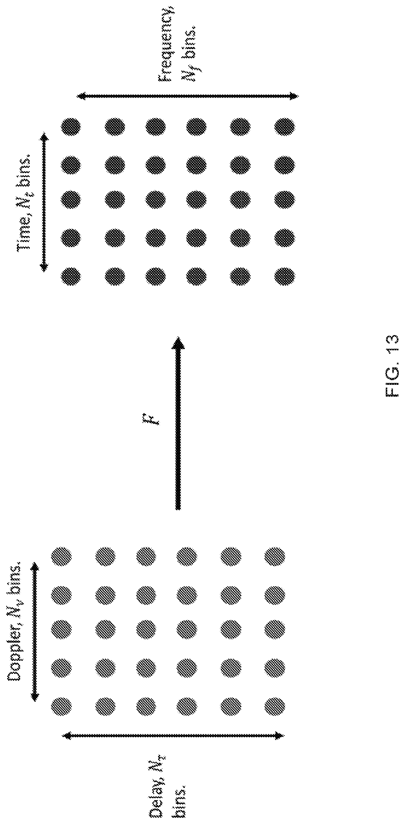
D00014
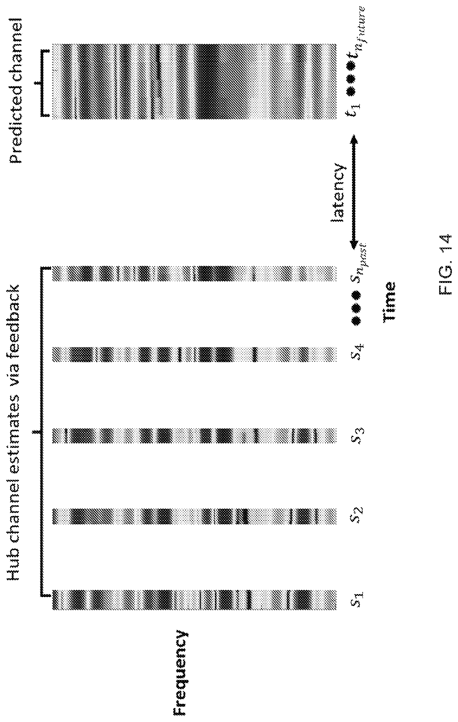
D00015
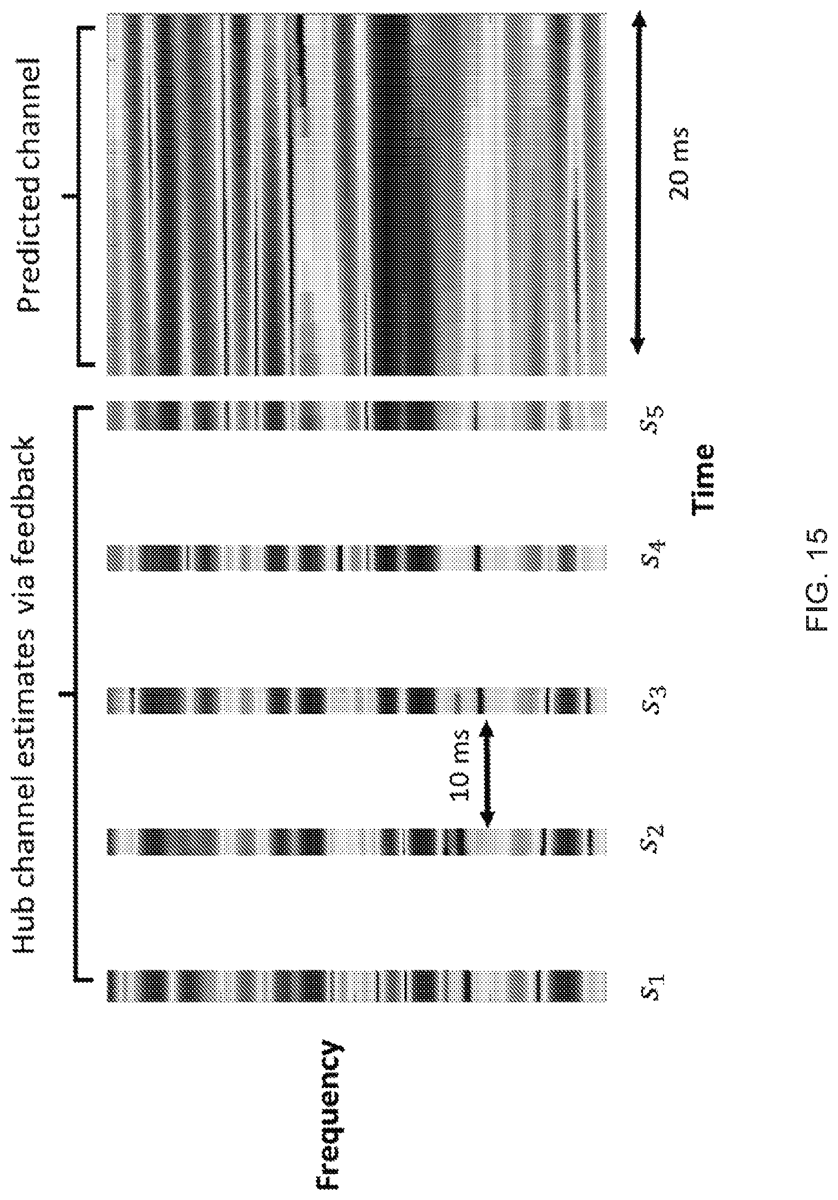
D00016
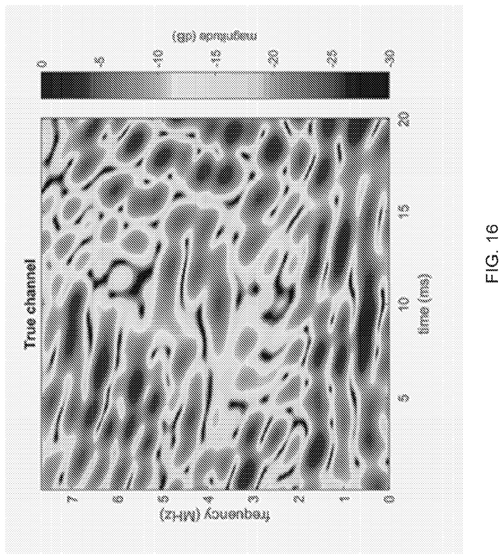
D00017

D00018
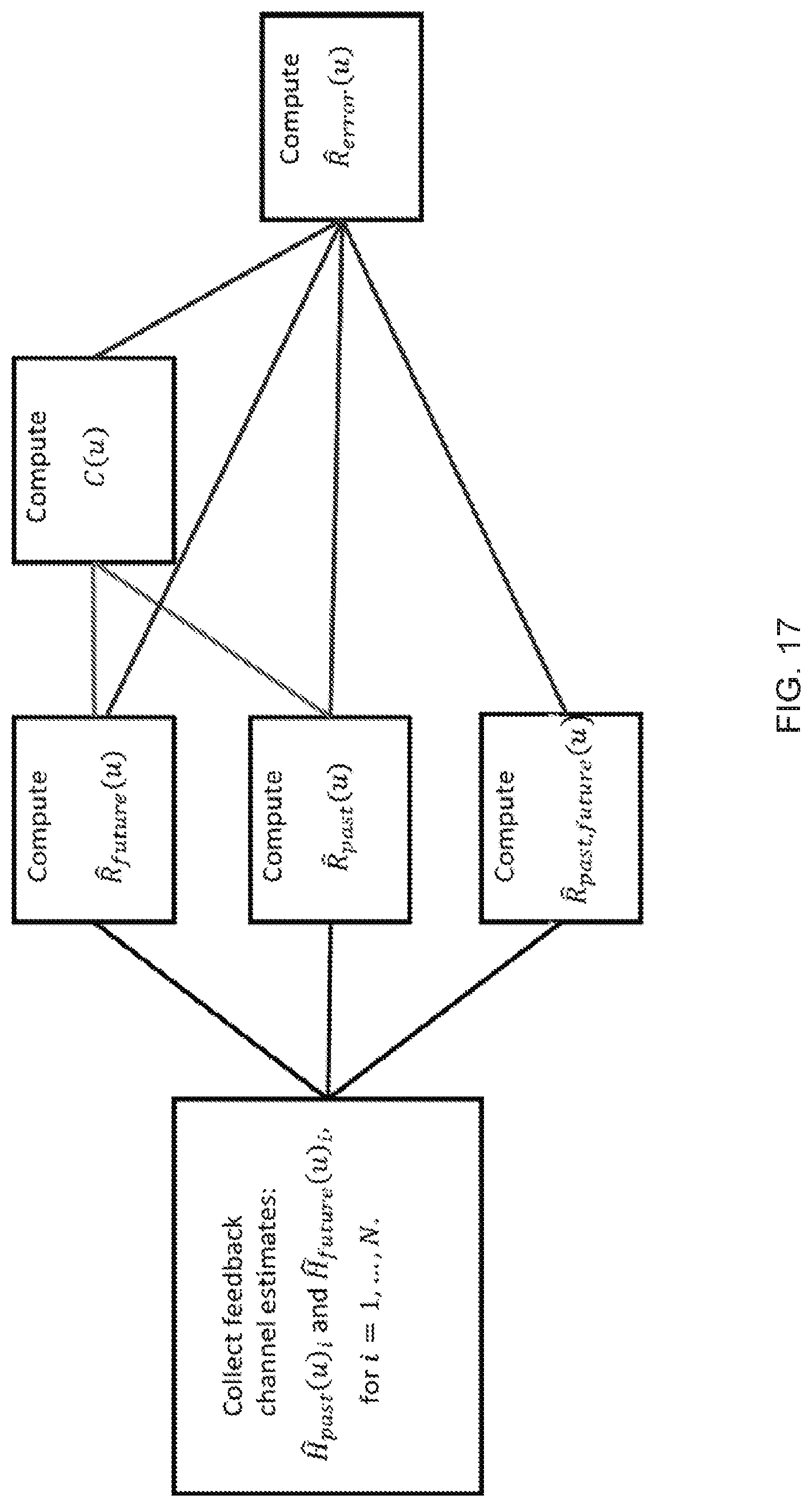
D00019
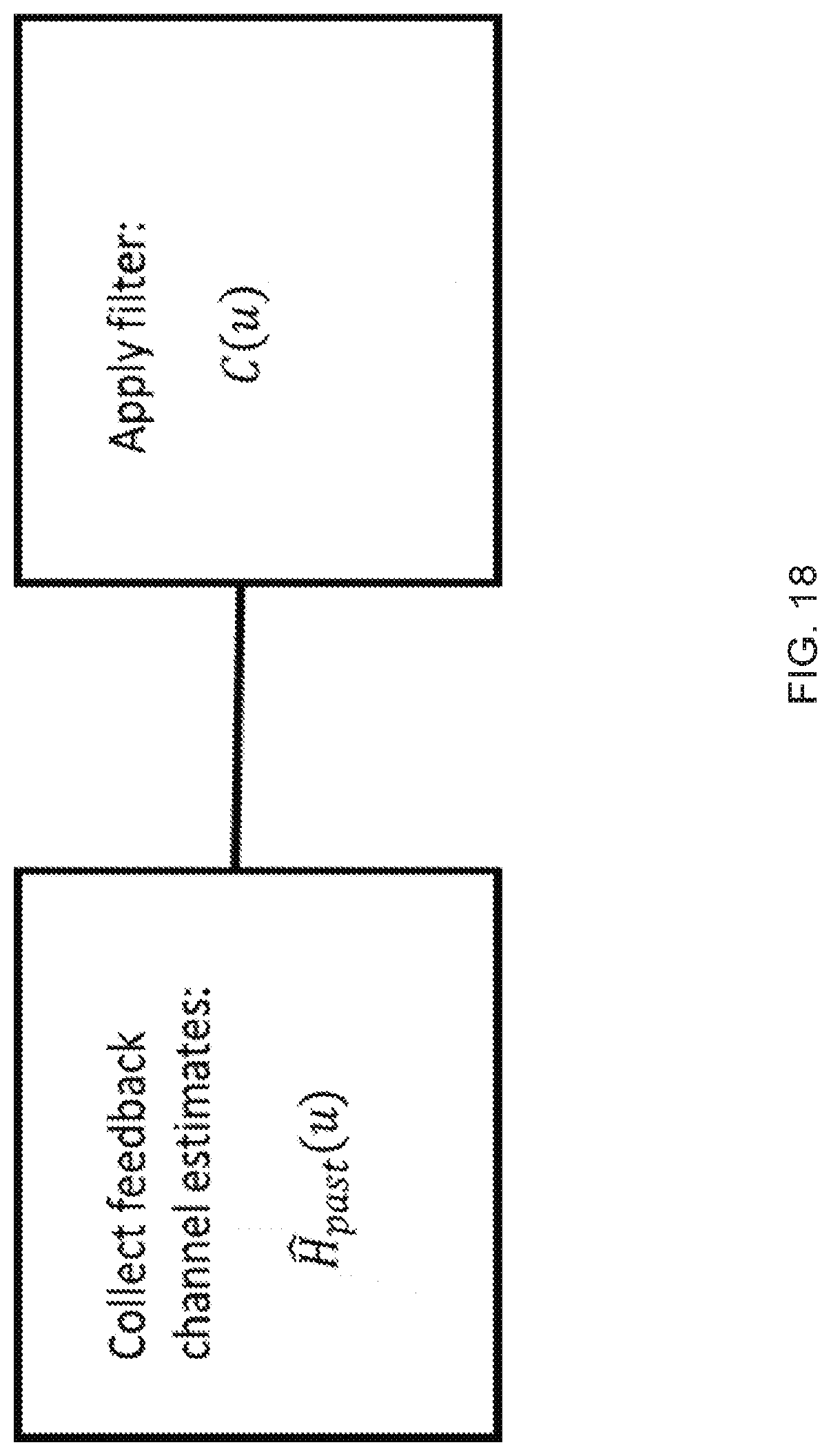
D00020
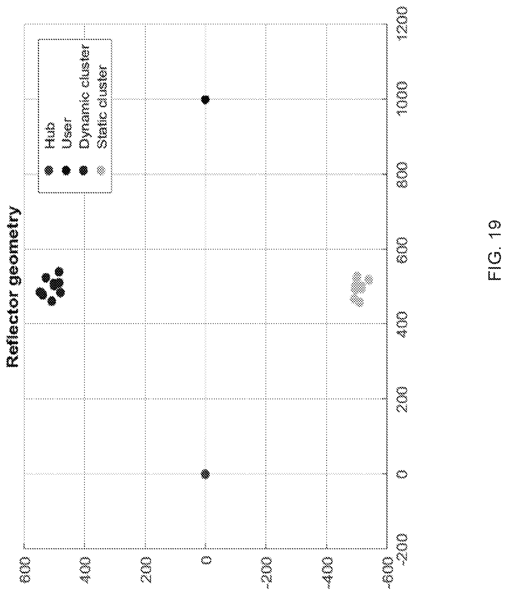
D00021

D00022
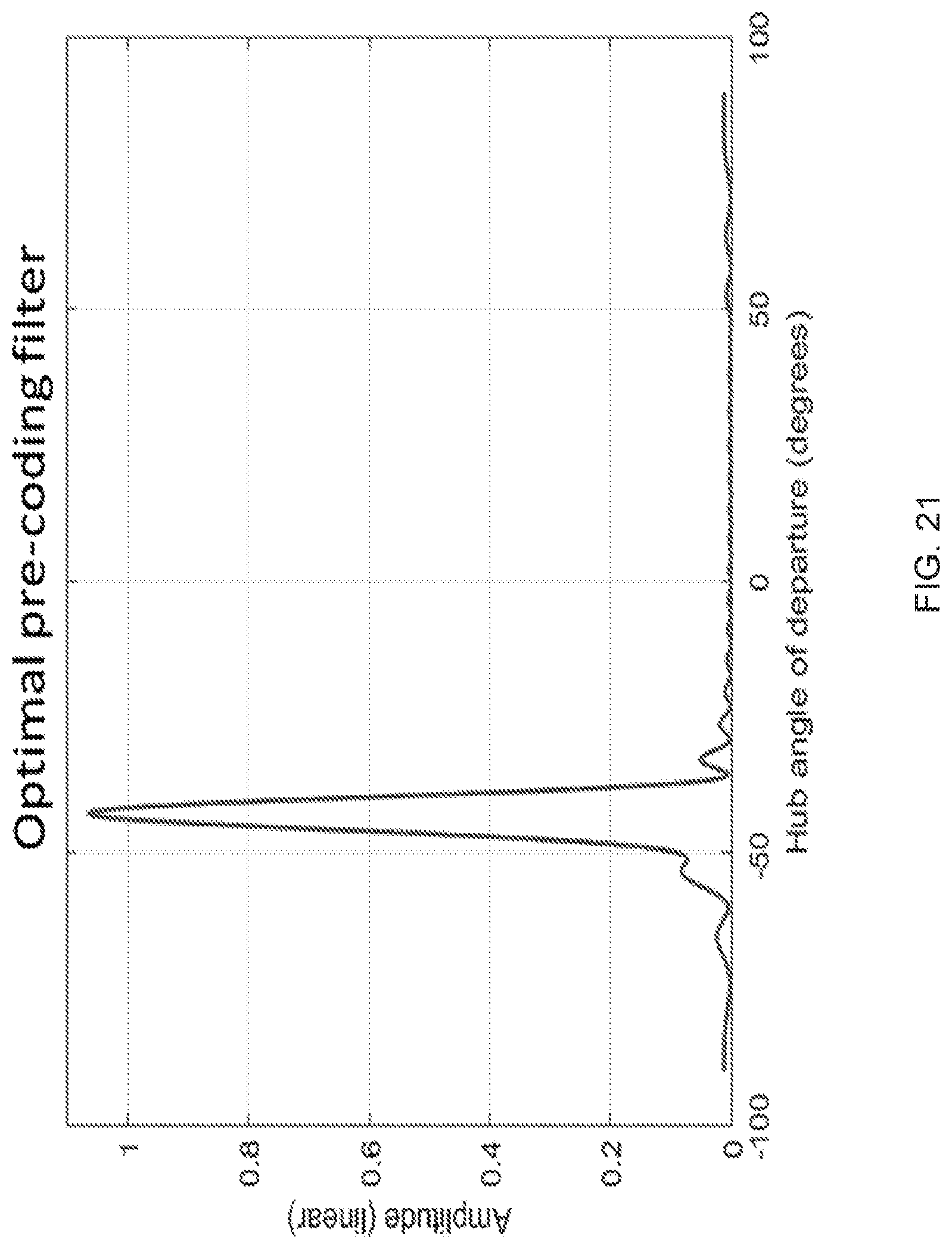
D00023
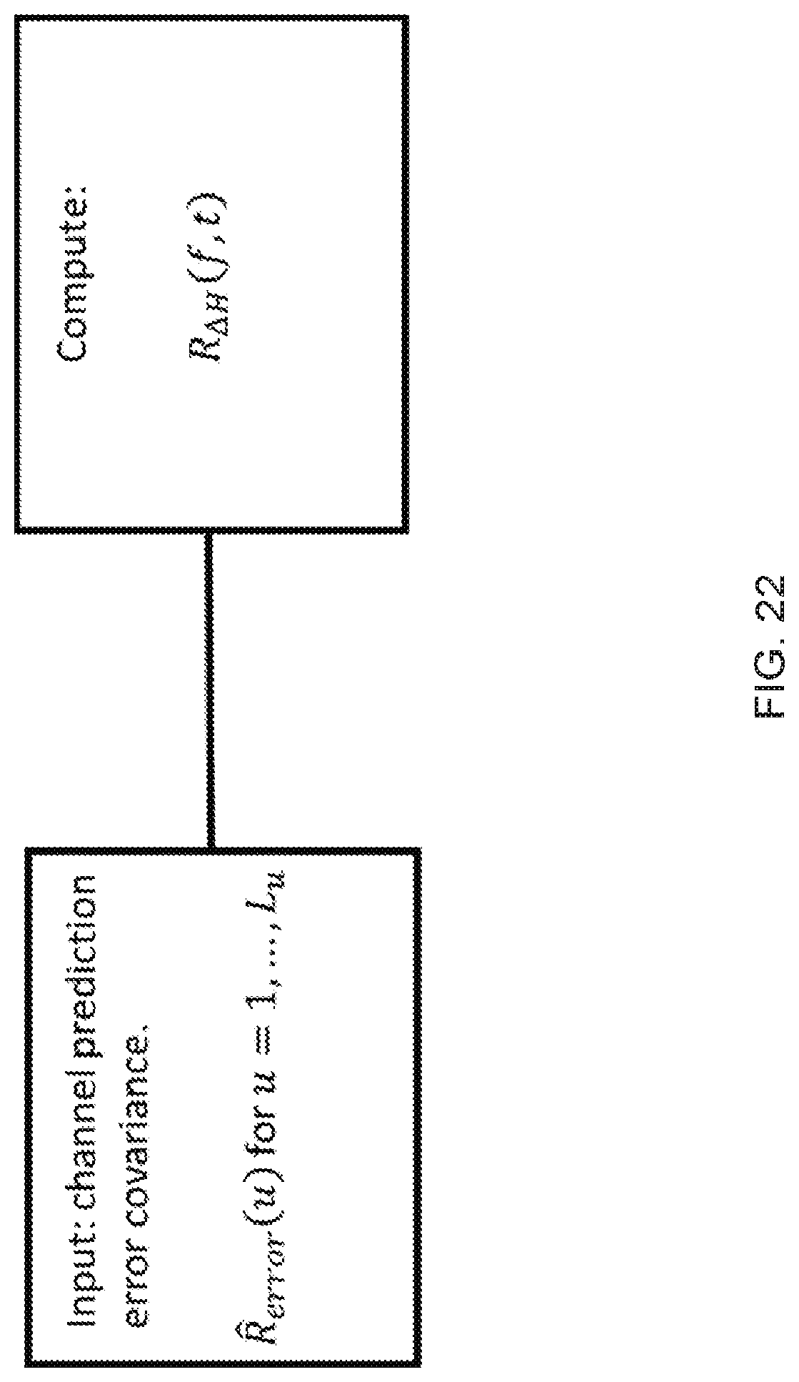
D00024
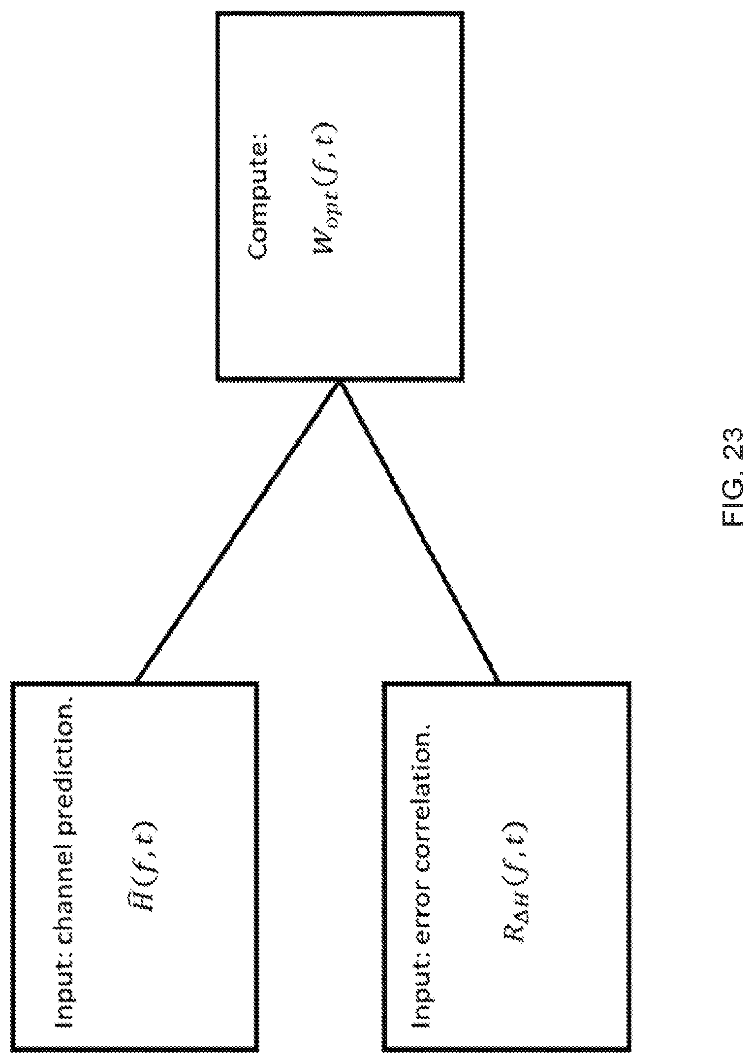
D00025
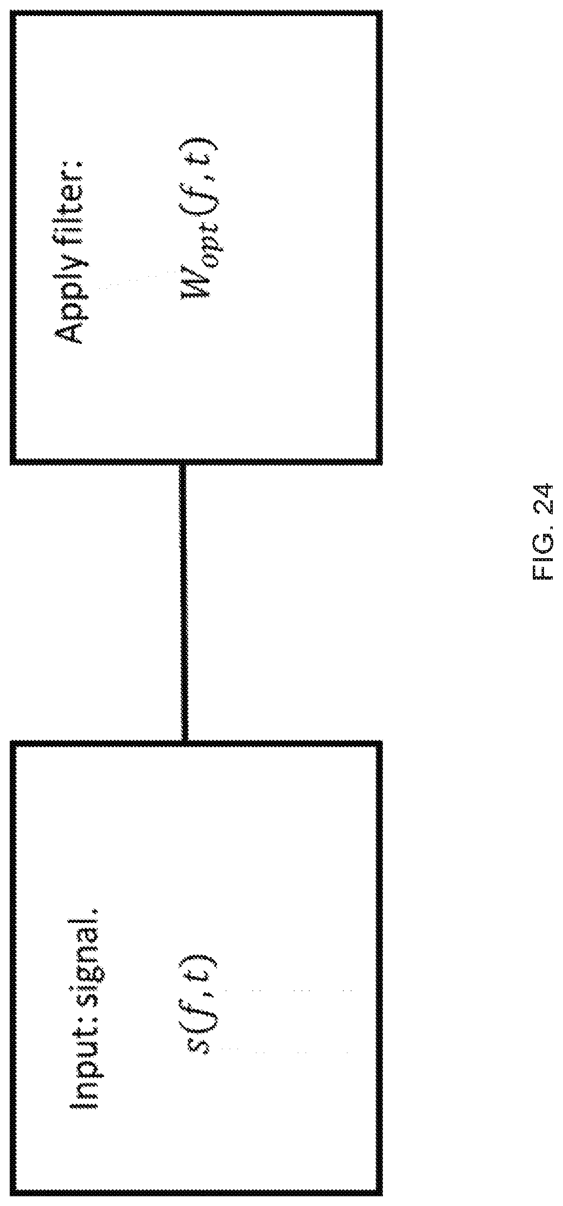
D00026
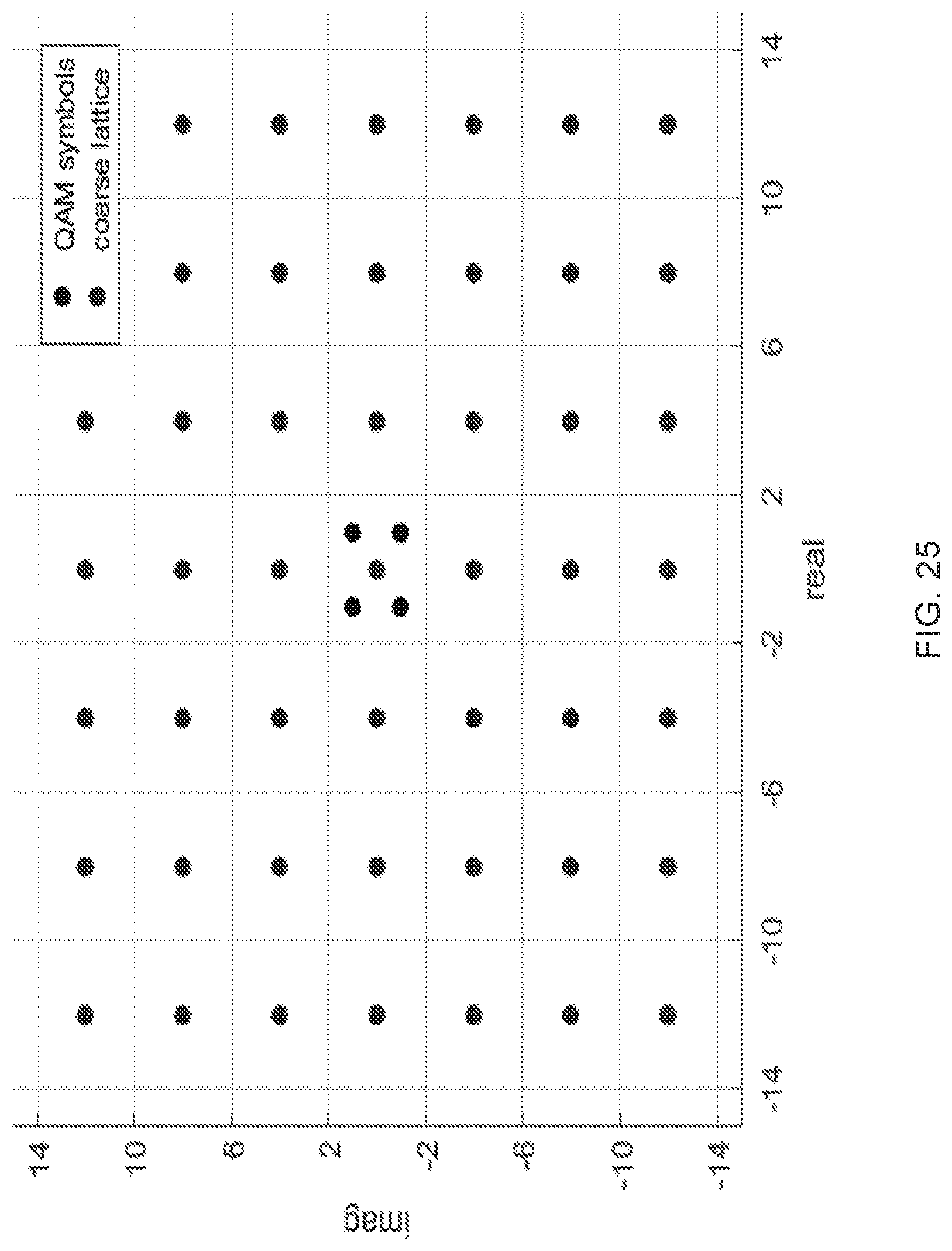
D00027
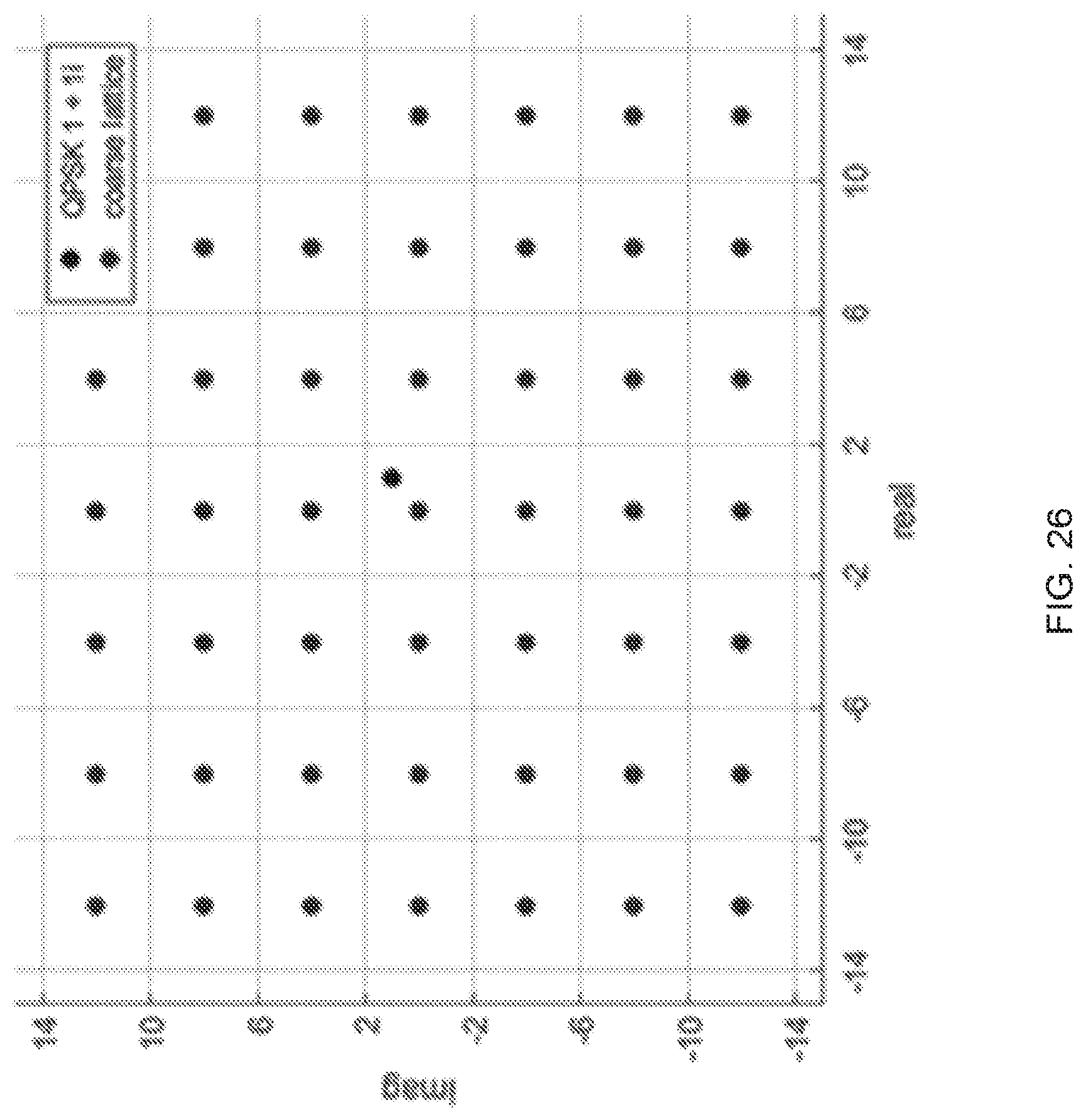
D00028
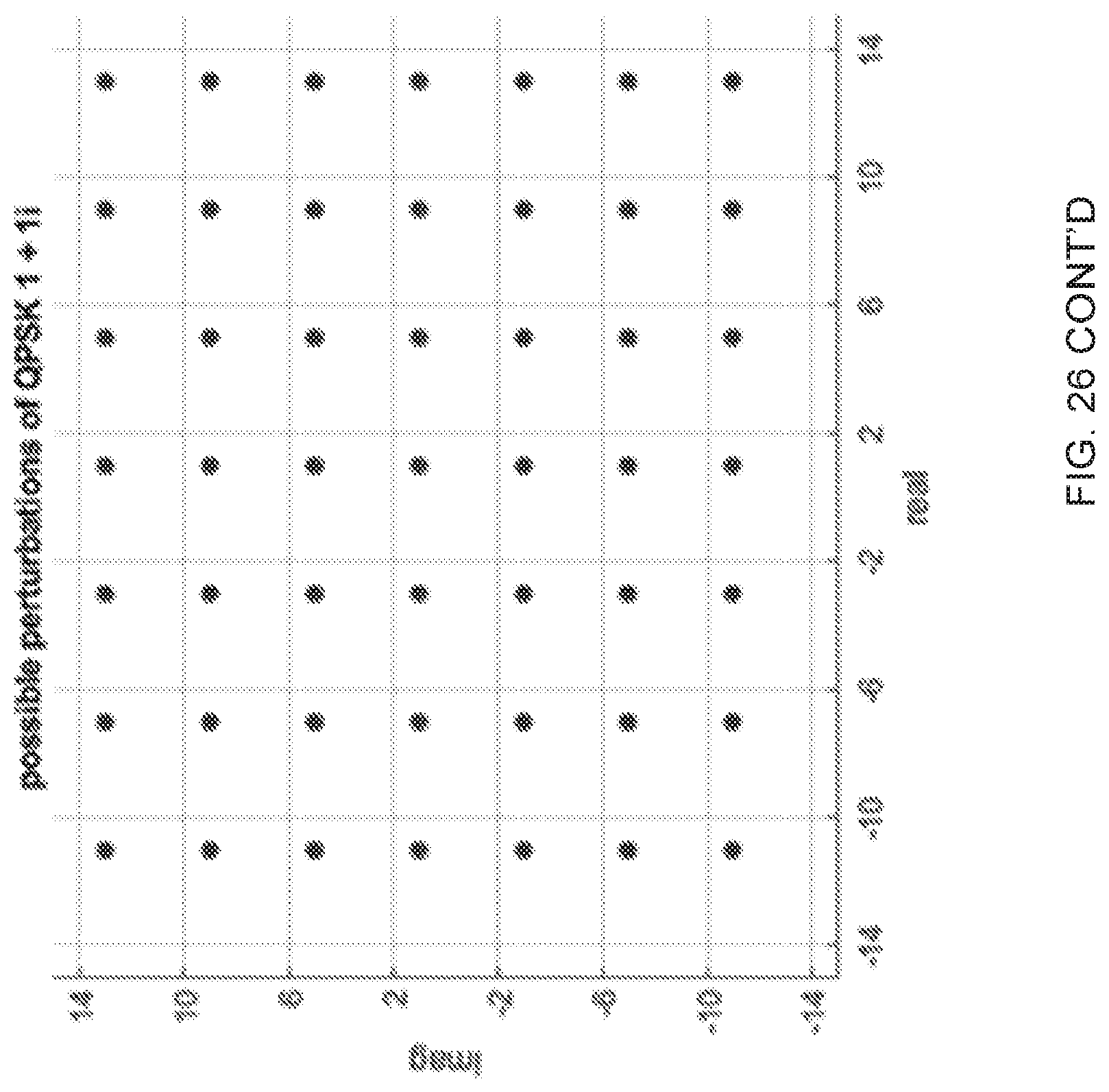
D00029
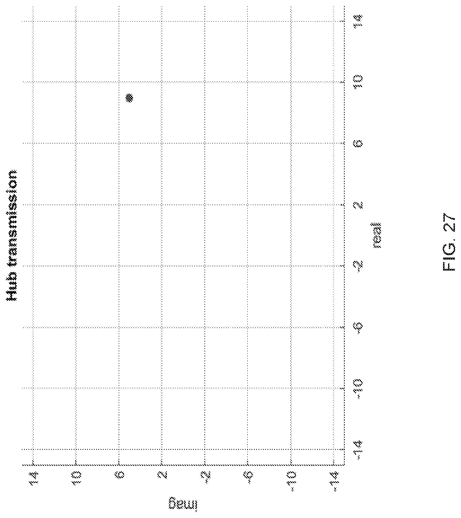
D00030
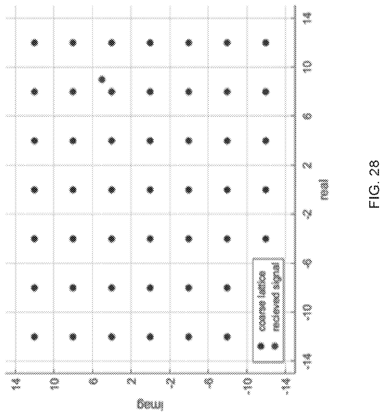
D00031
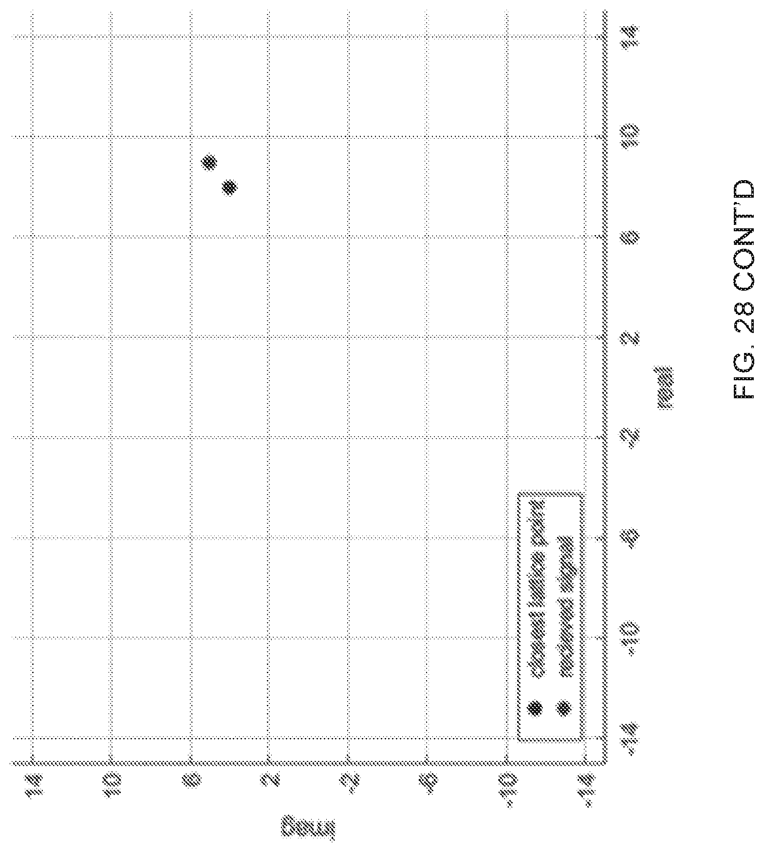
D00032
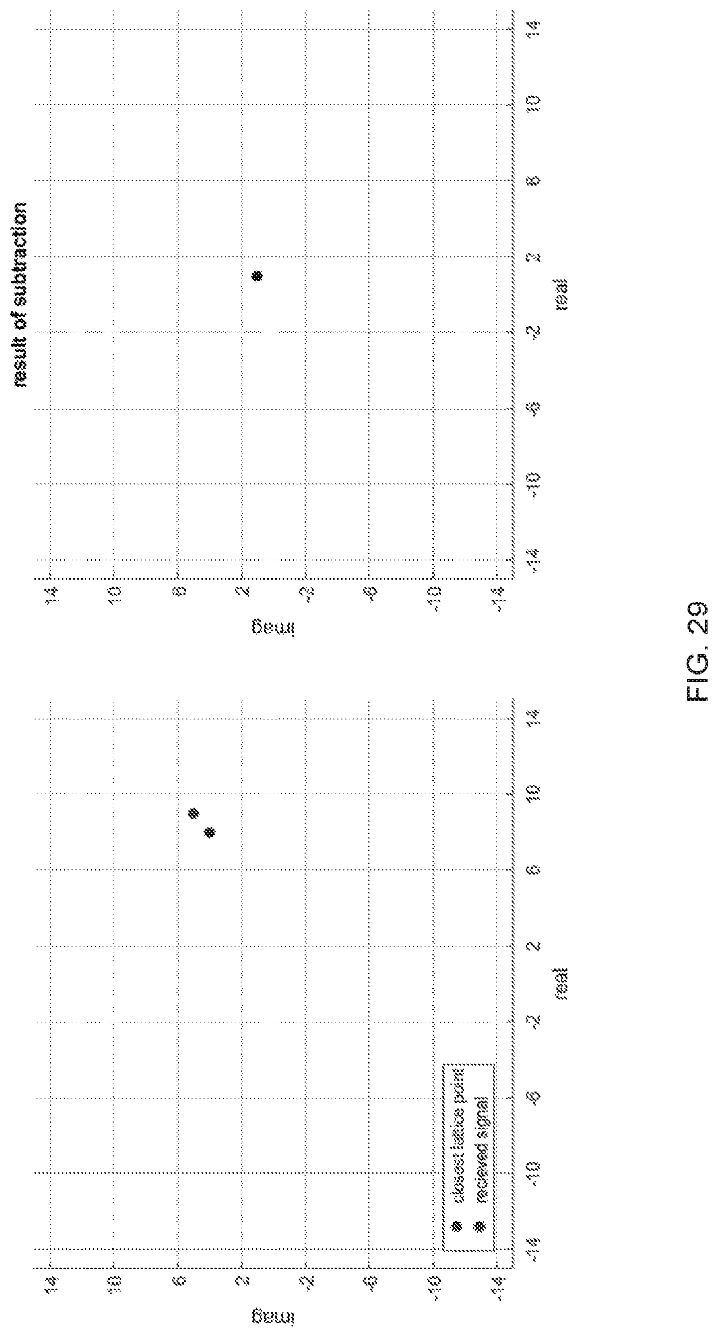
D00033
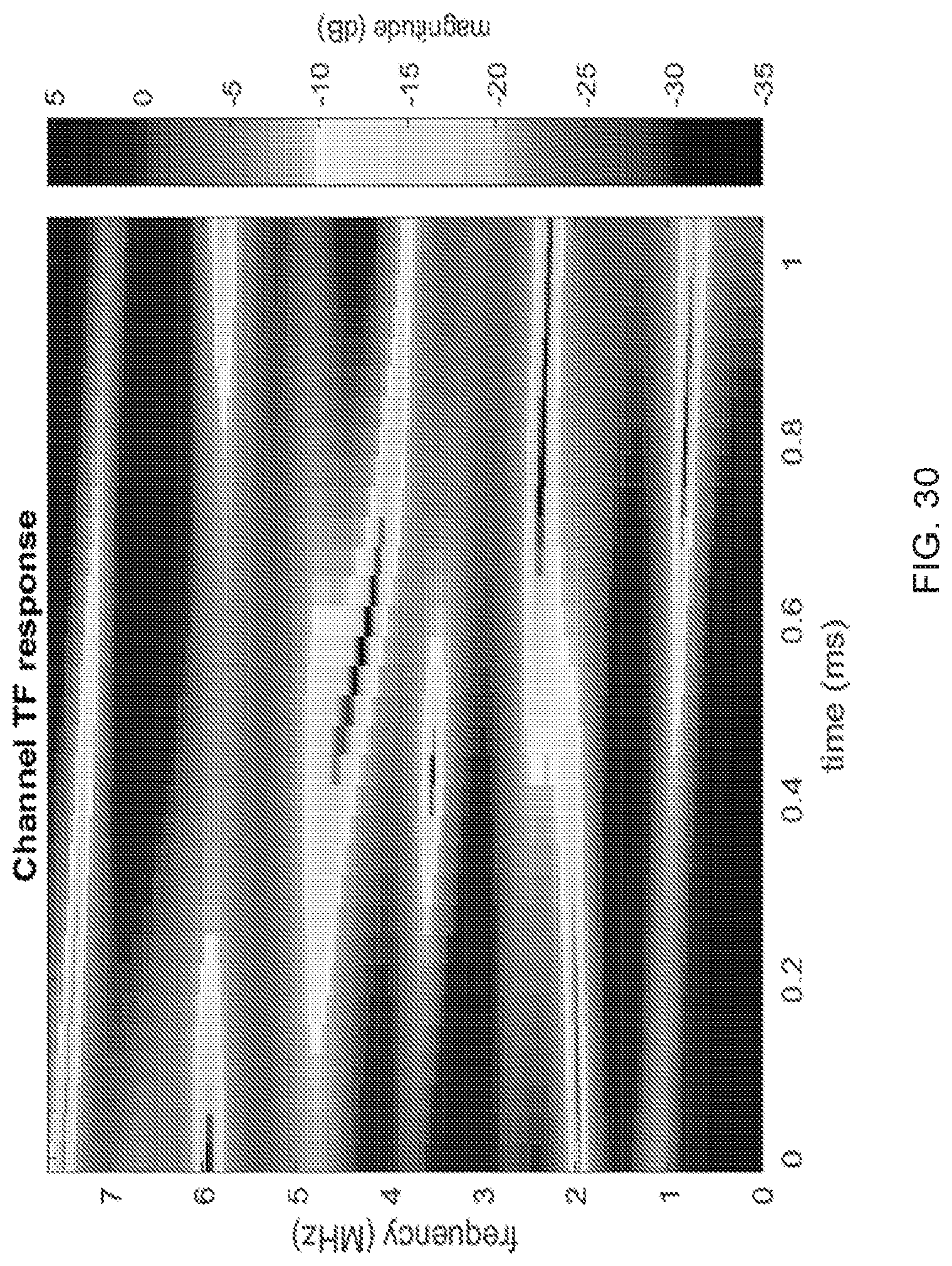
D00034

D00035
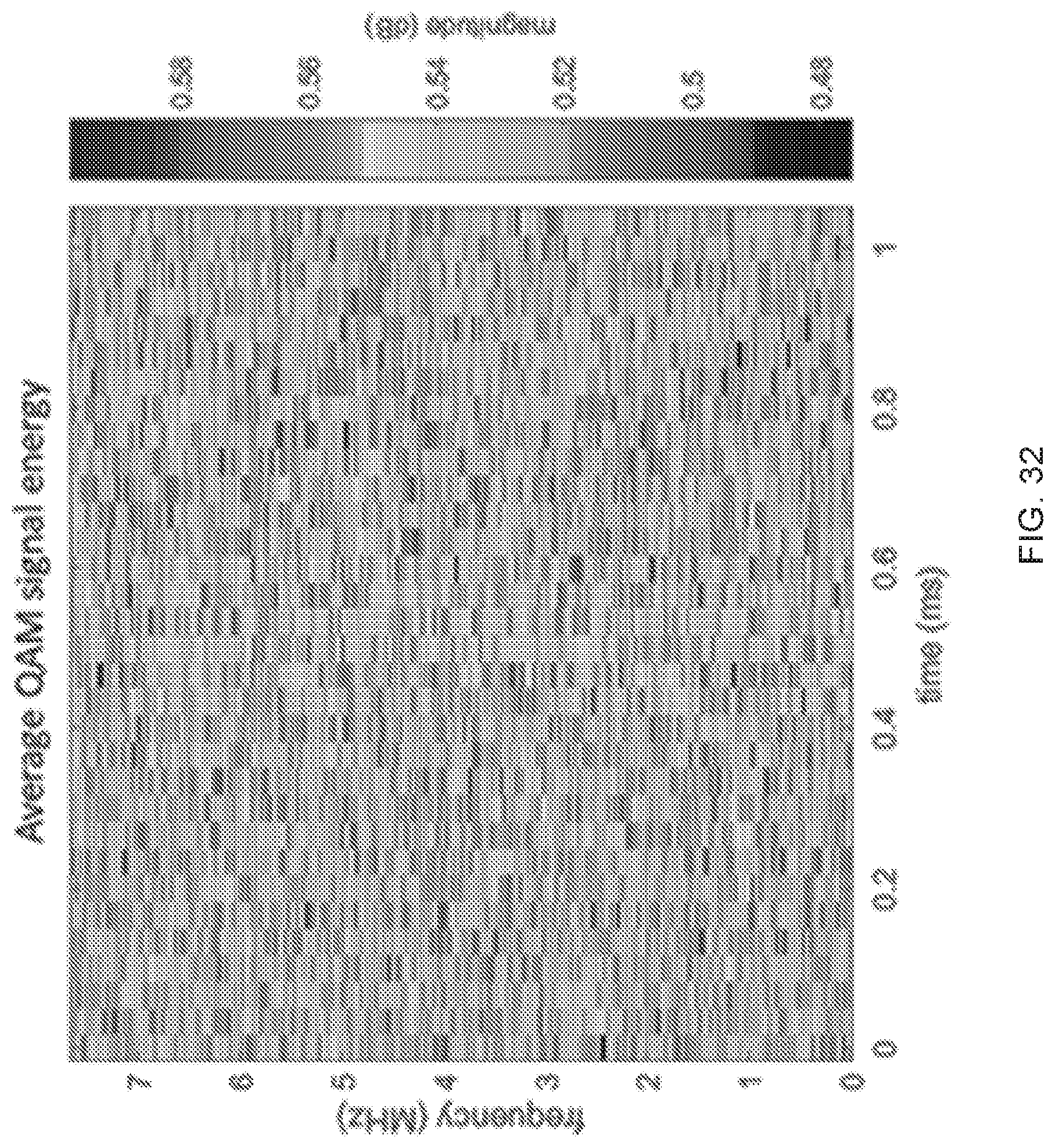
D00036
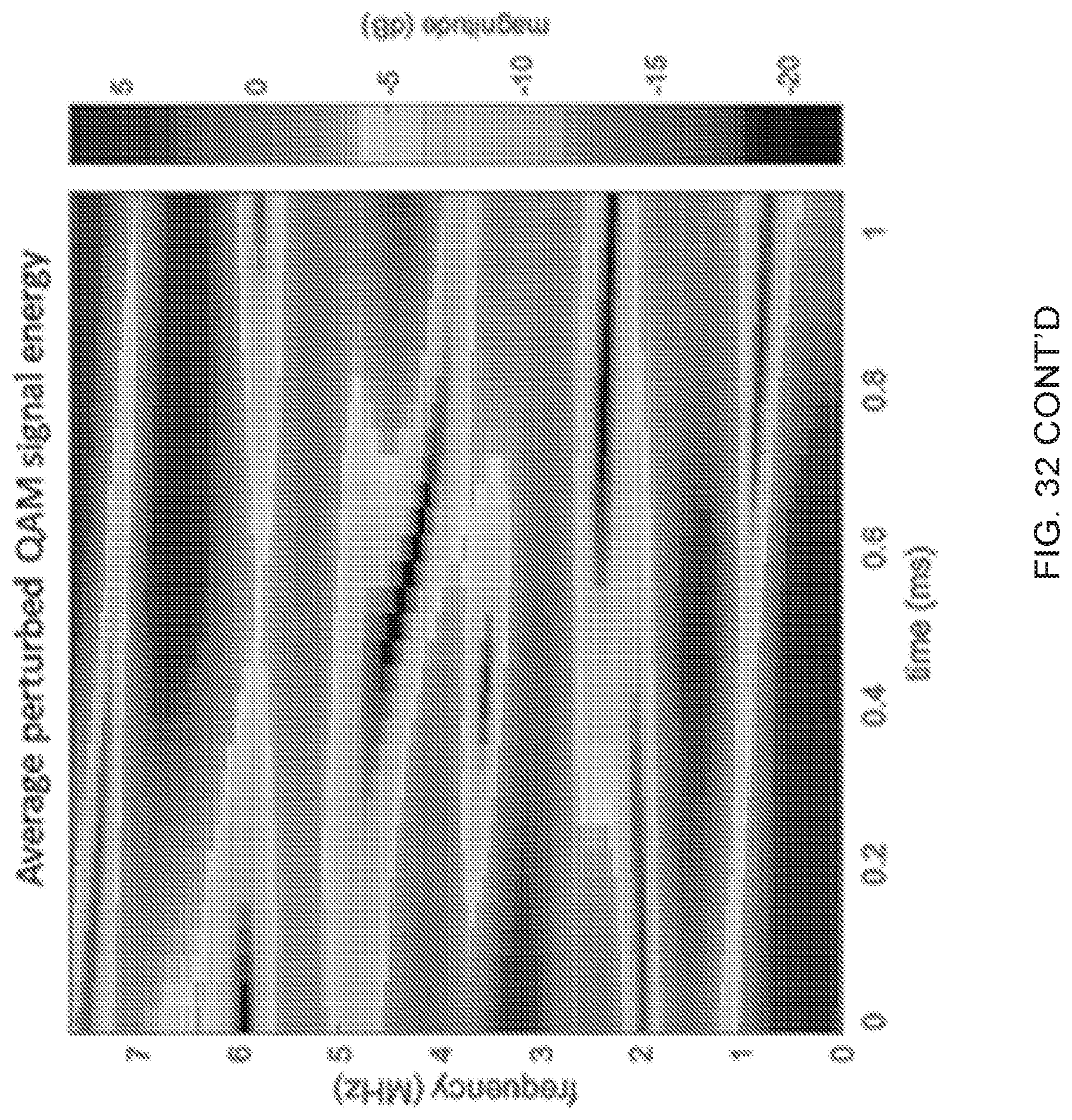
D00037
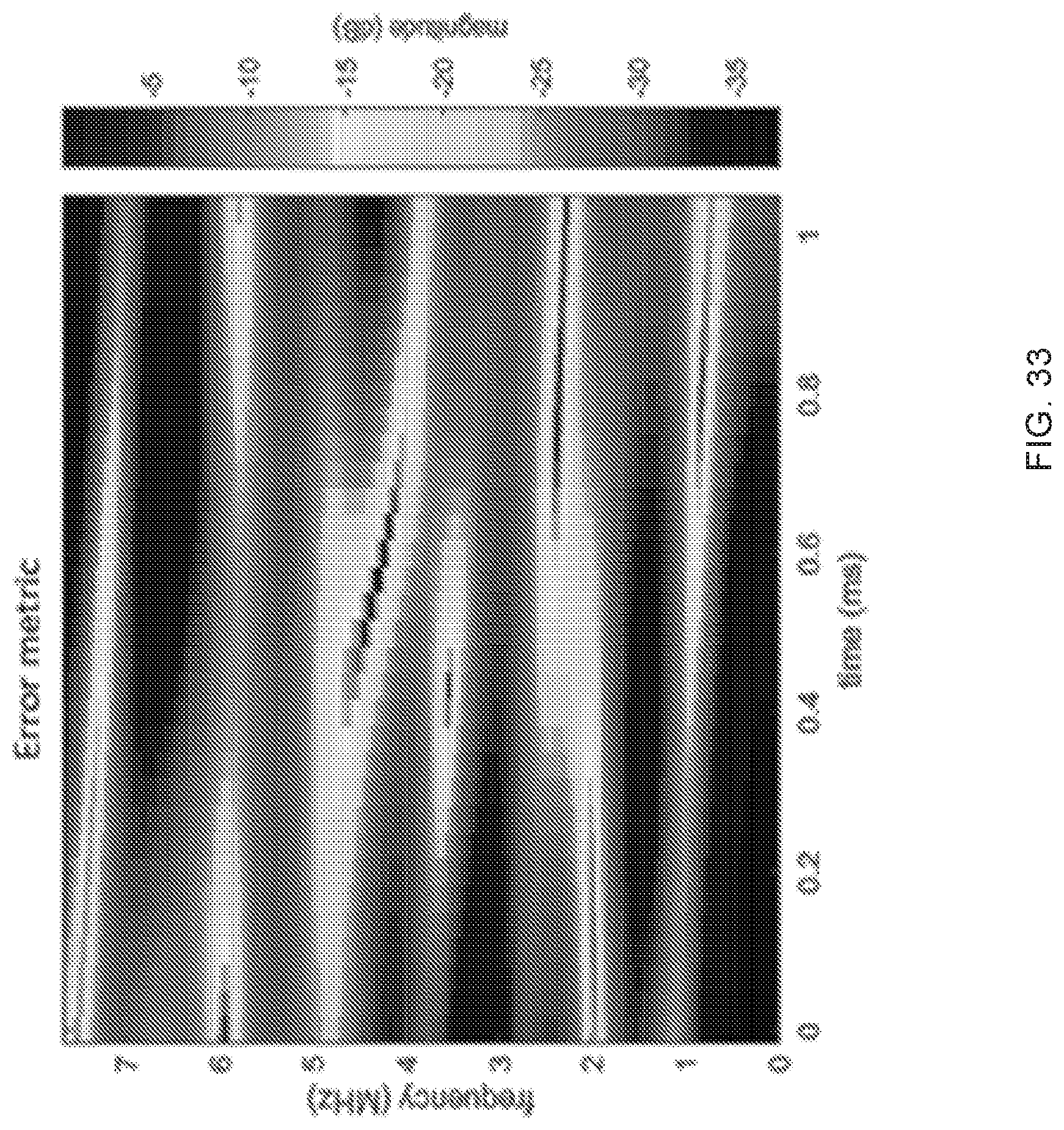
D00038

D00039
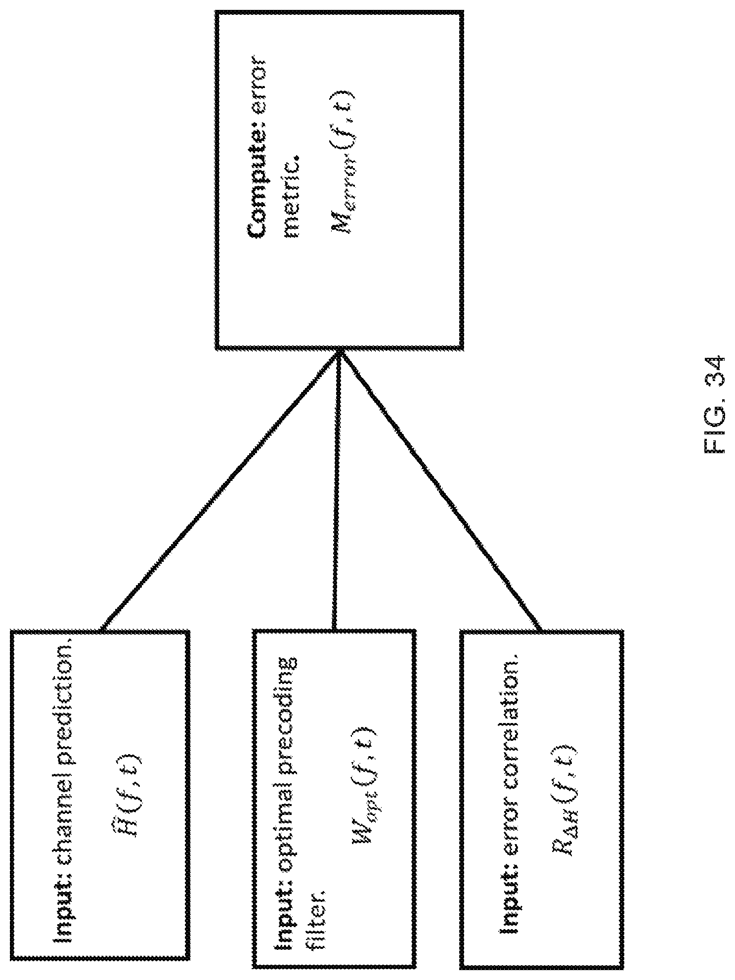
D00040
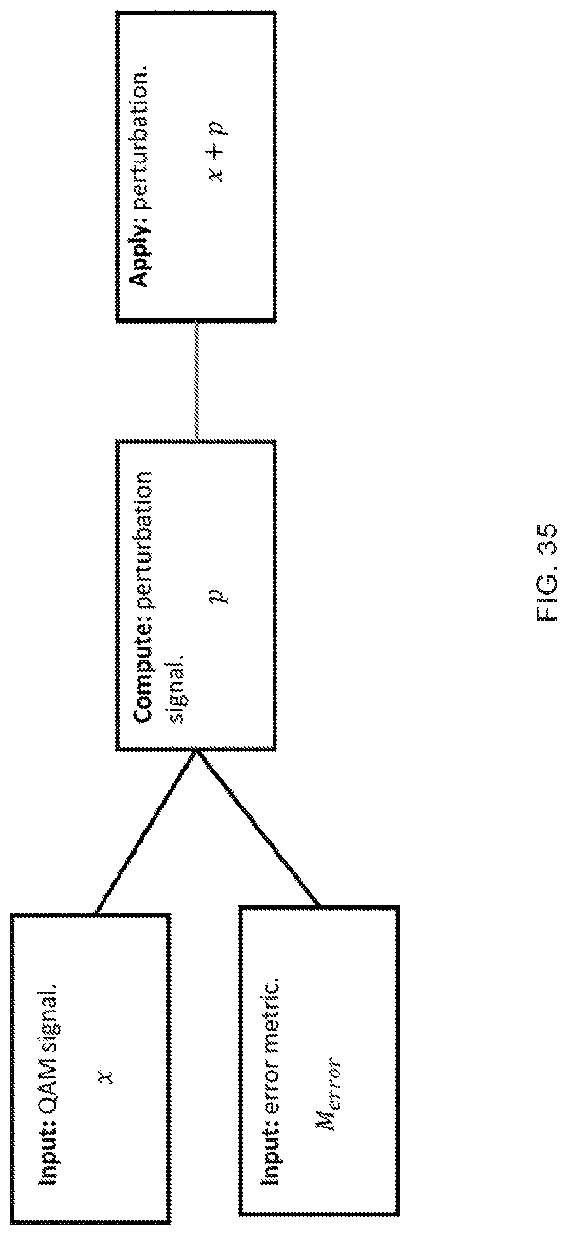
D00041
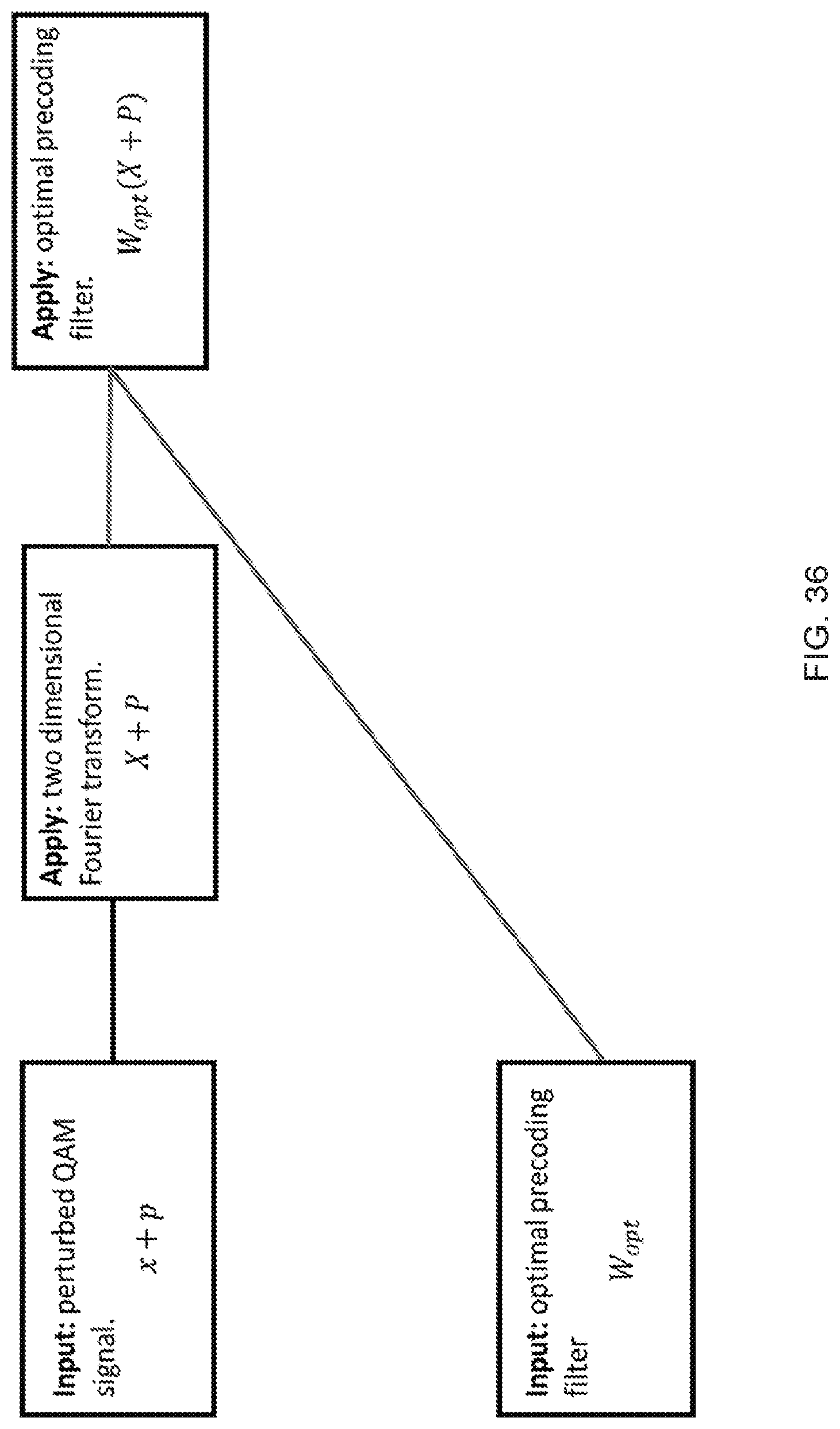
D00042
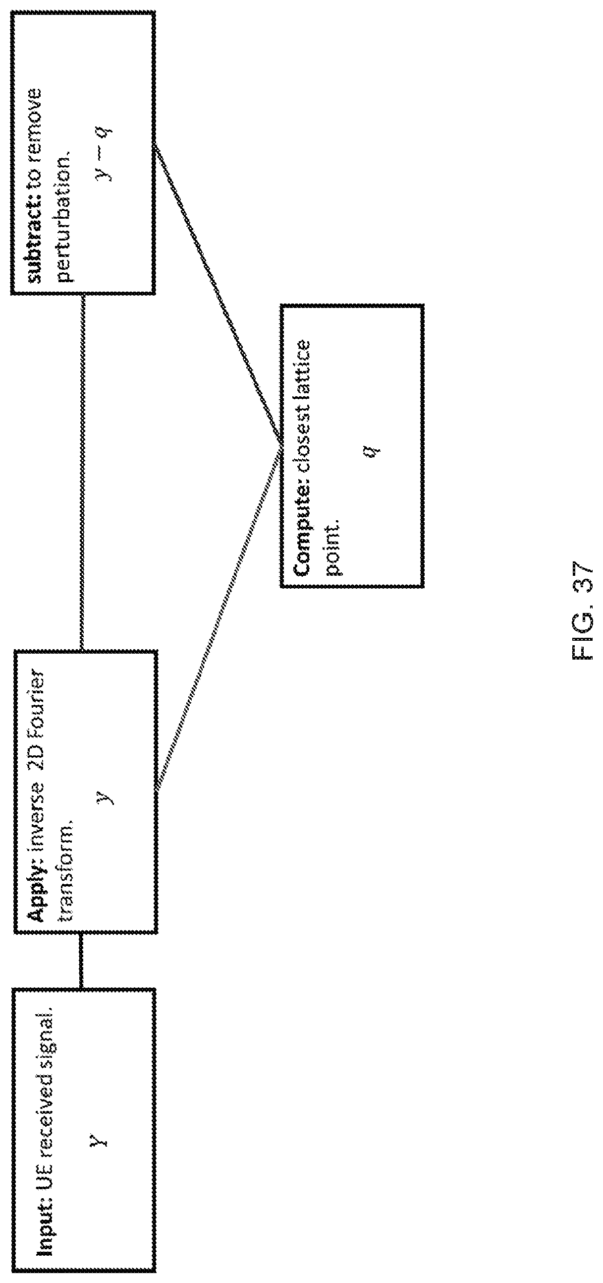
D00043
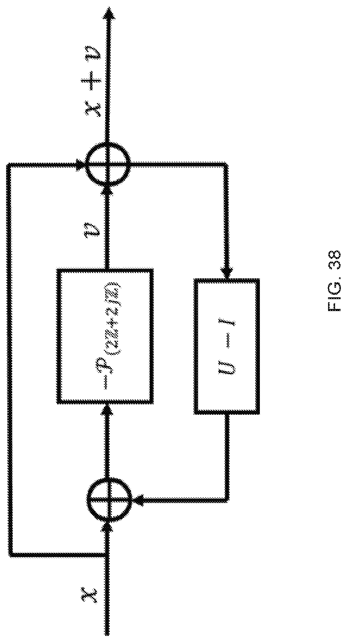
D00044
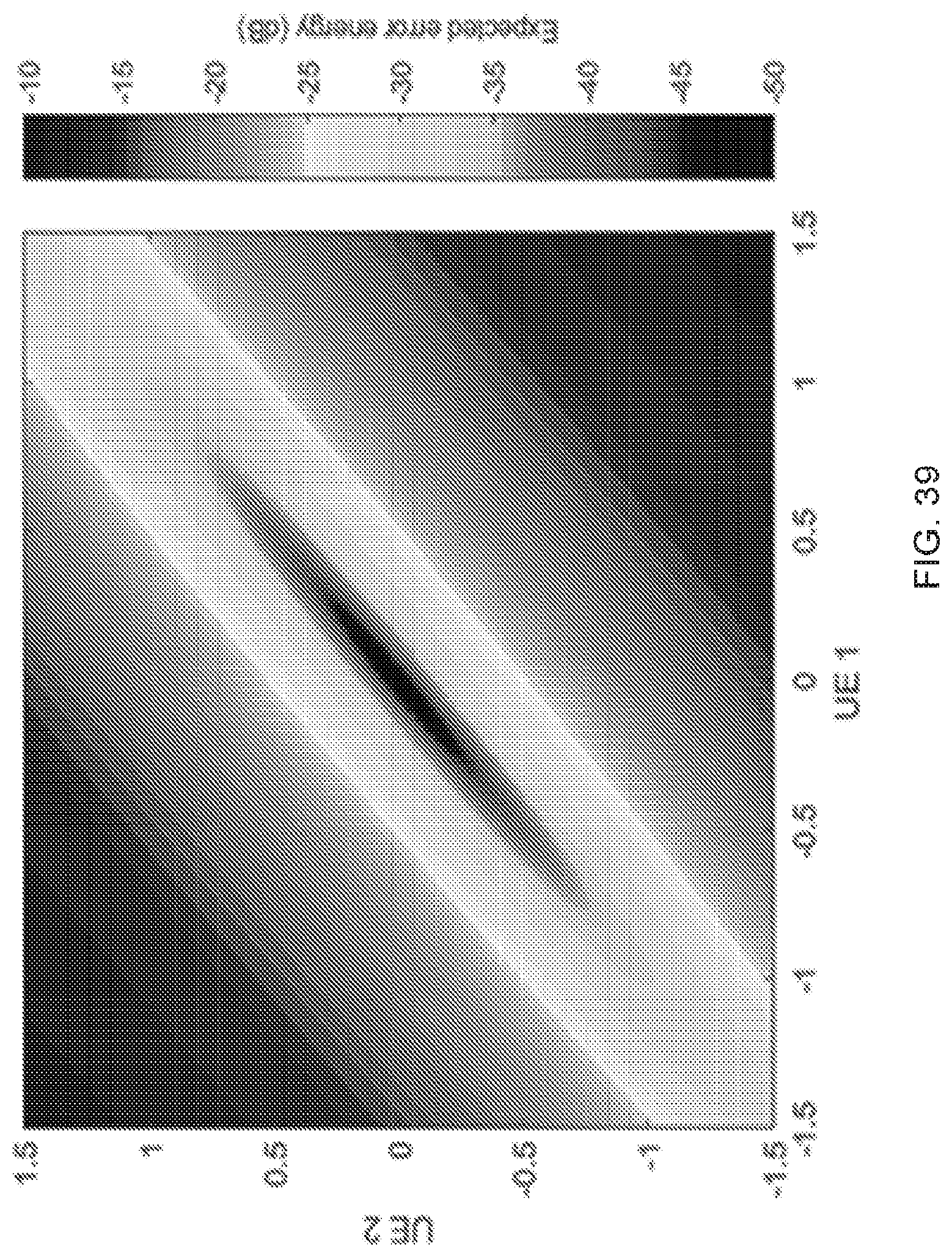
D00045
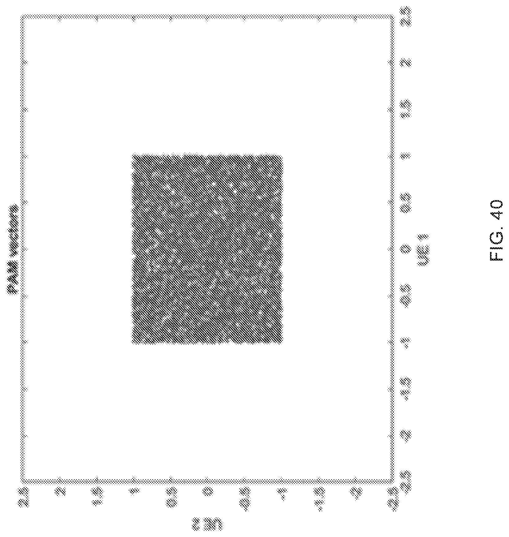
D00046
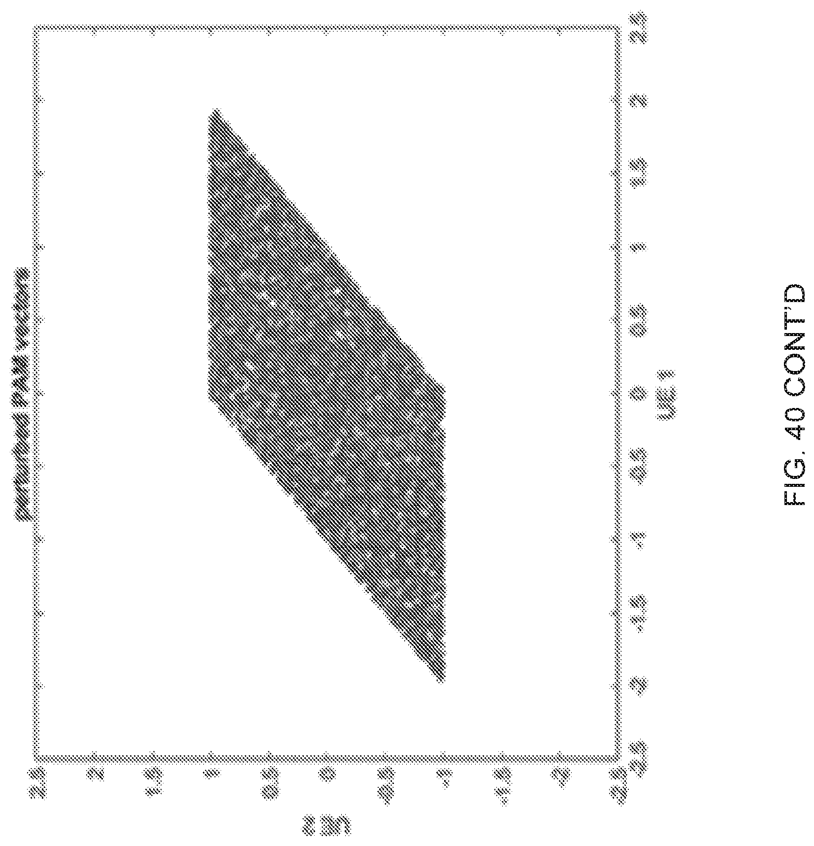
D00047
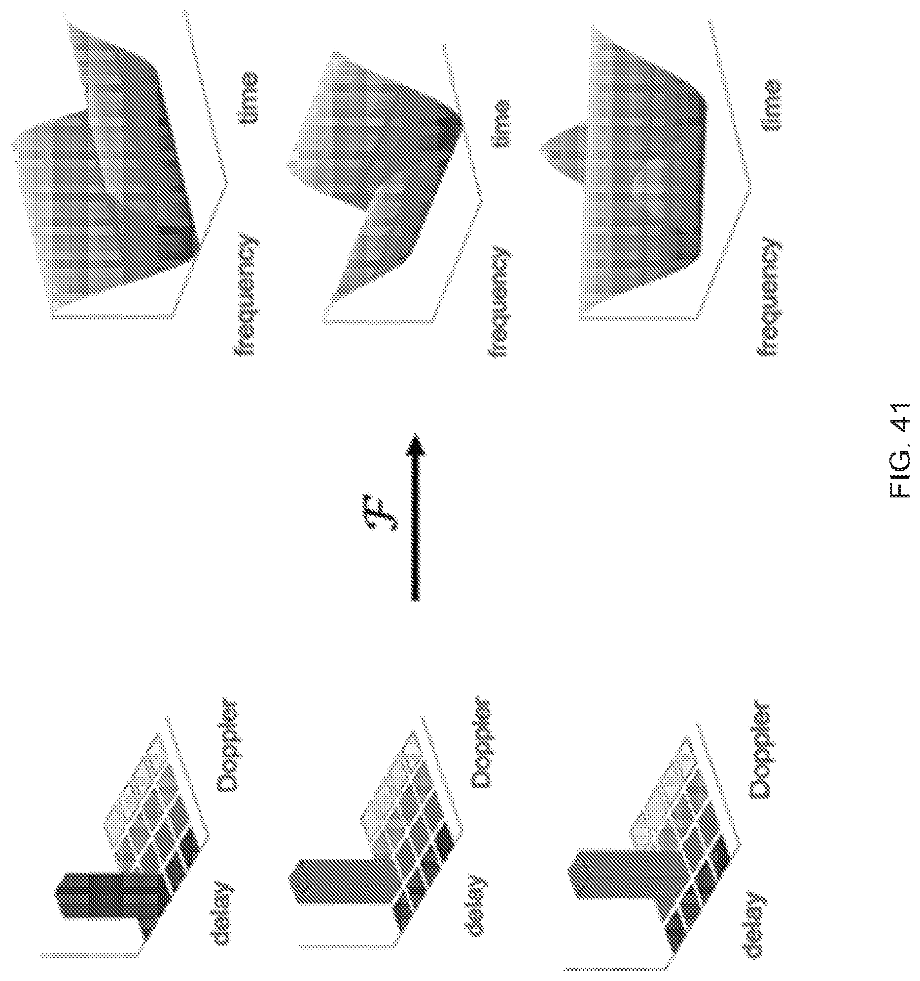
D00048

D00049
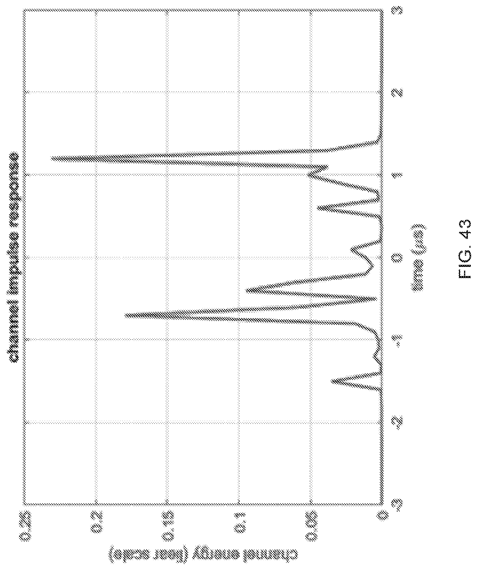
D00050
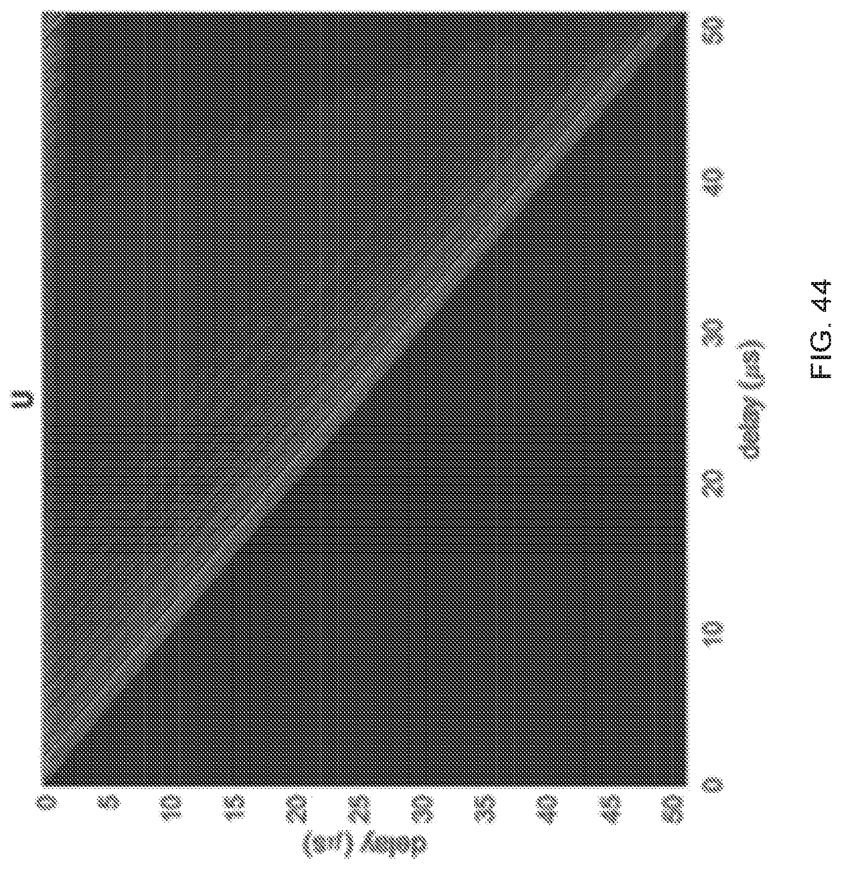
D00051
D00052
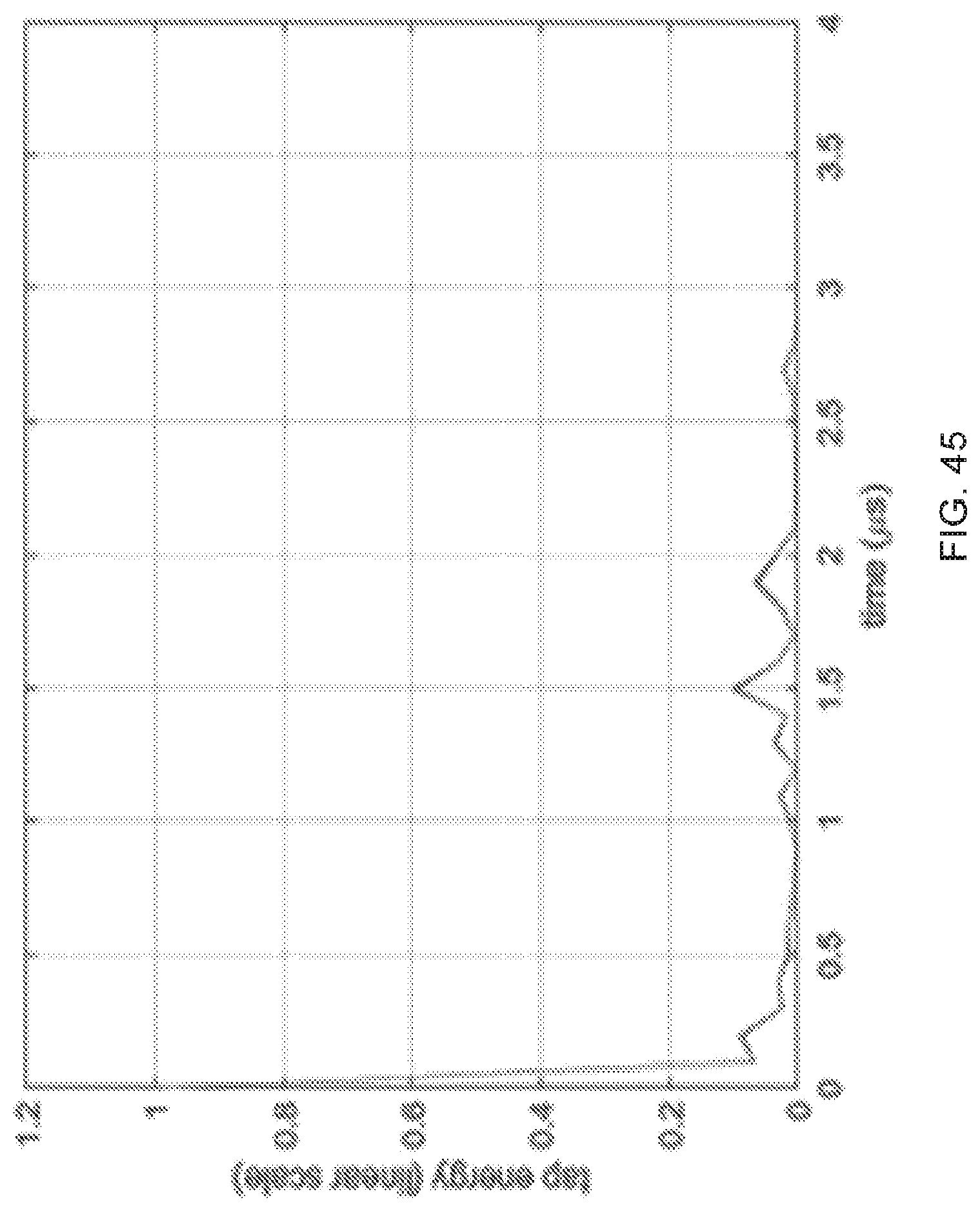
D00053
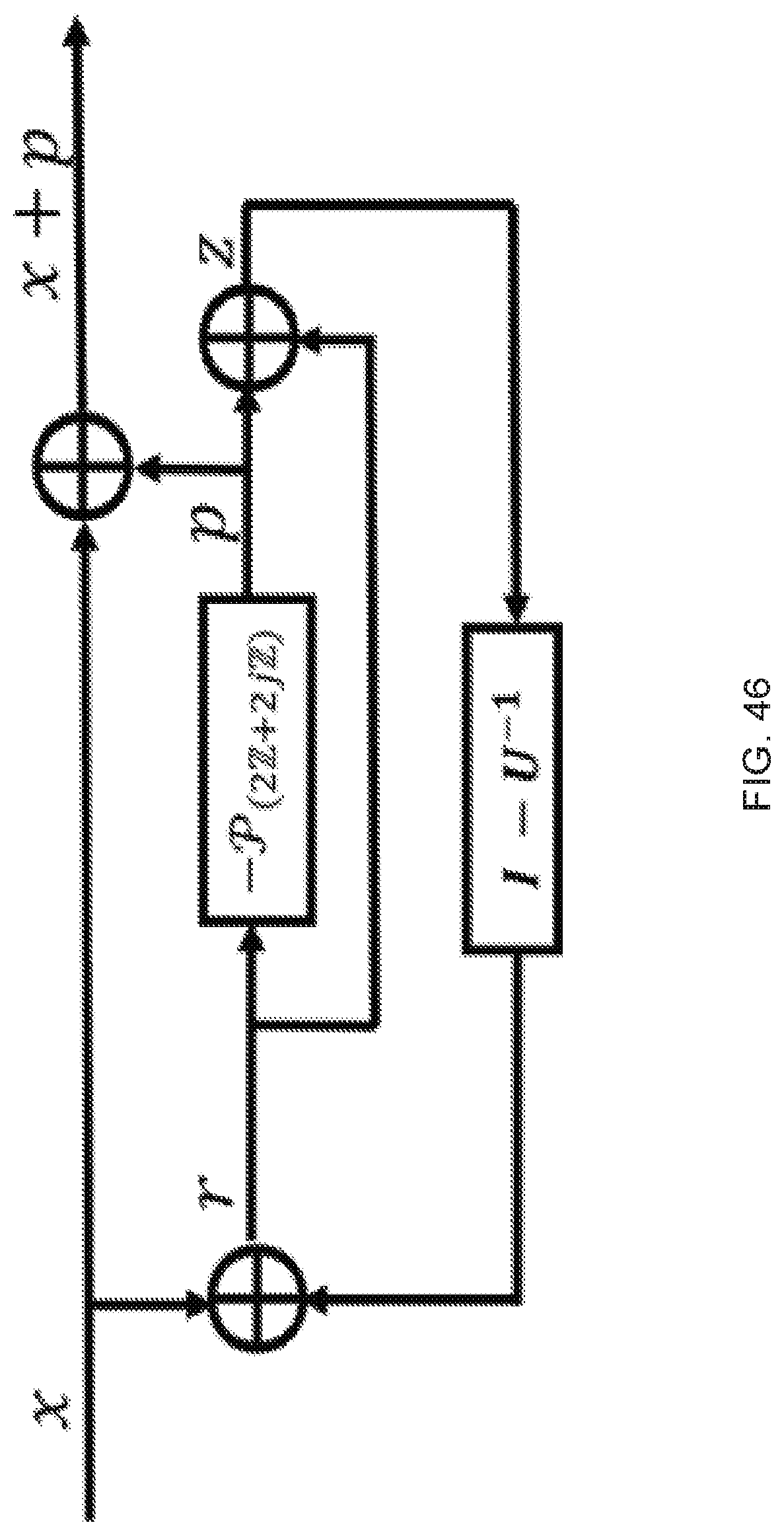
D00054
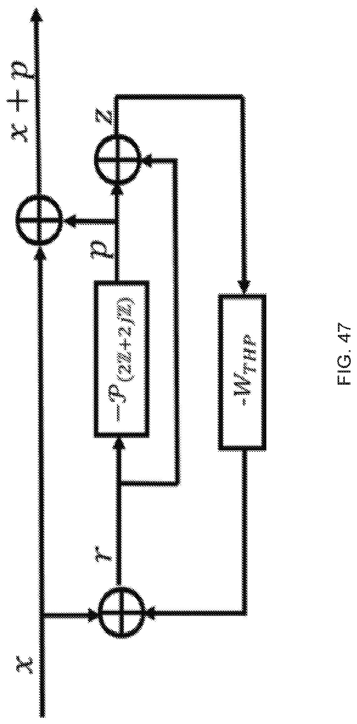
D00055
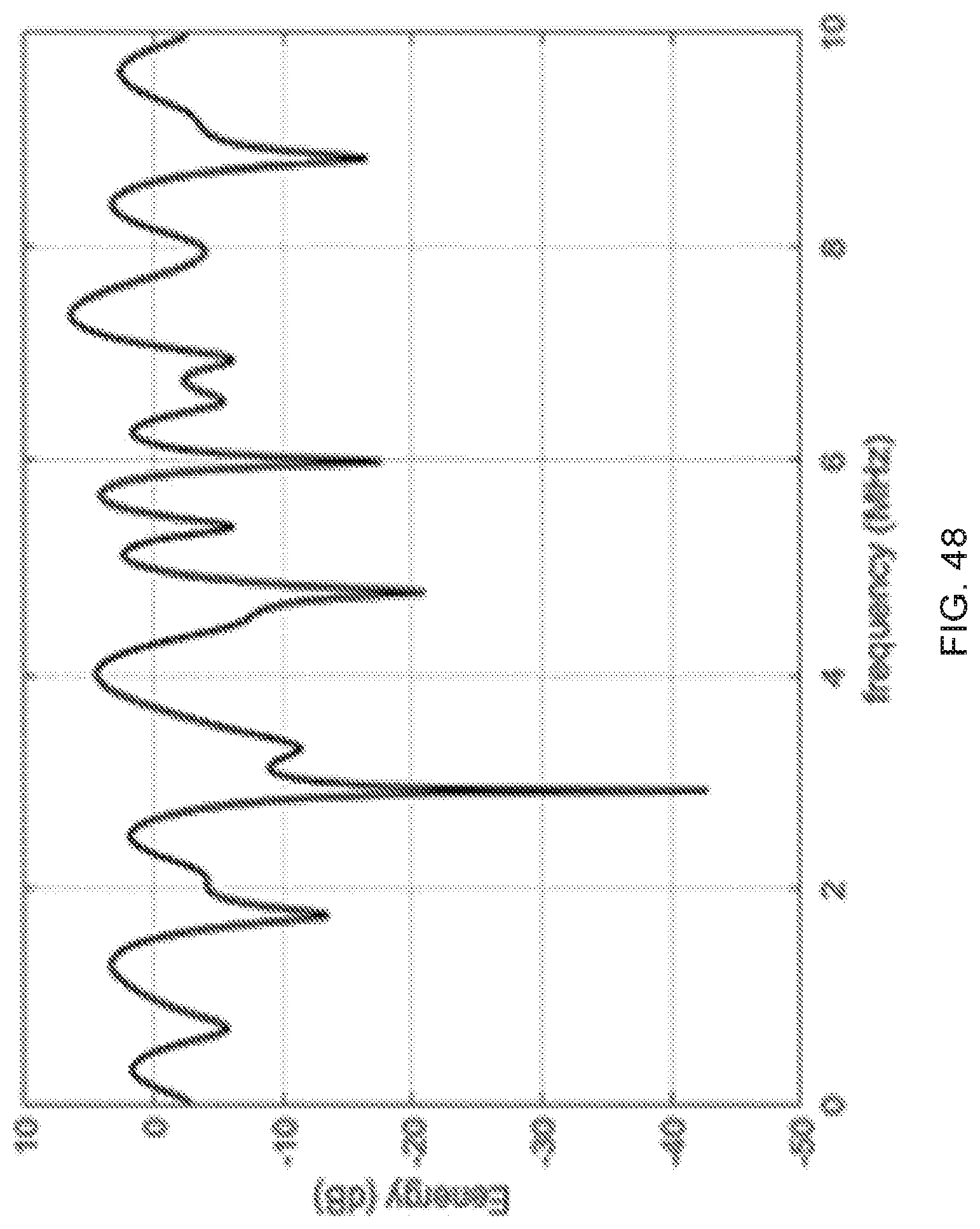
D00056
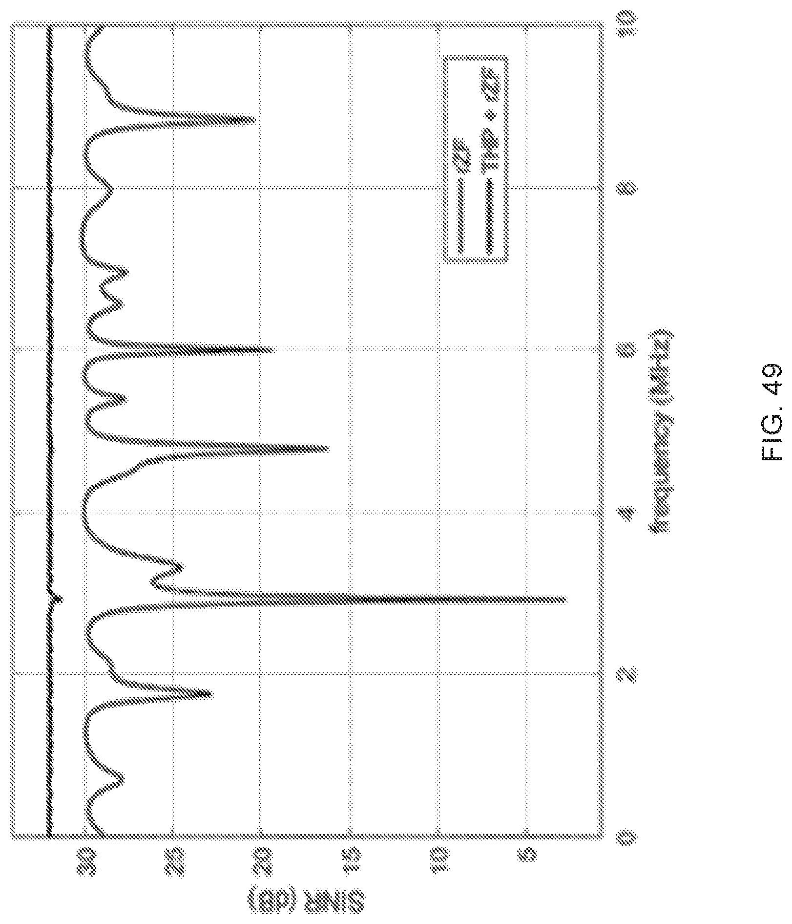
D00057
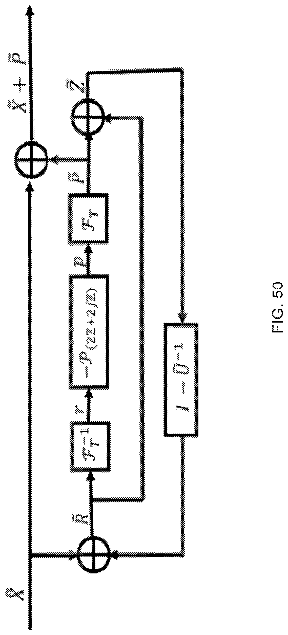
D00058
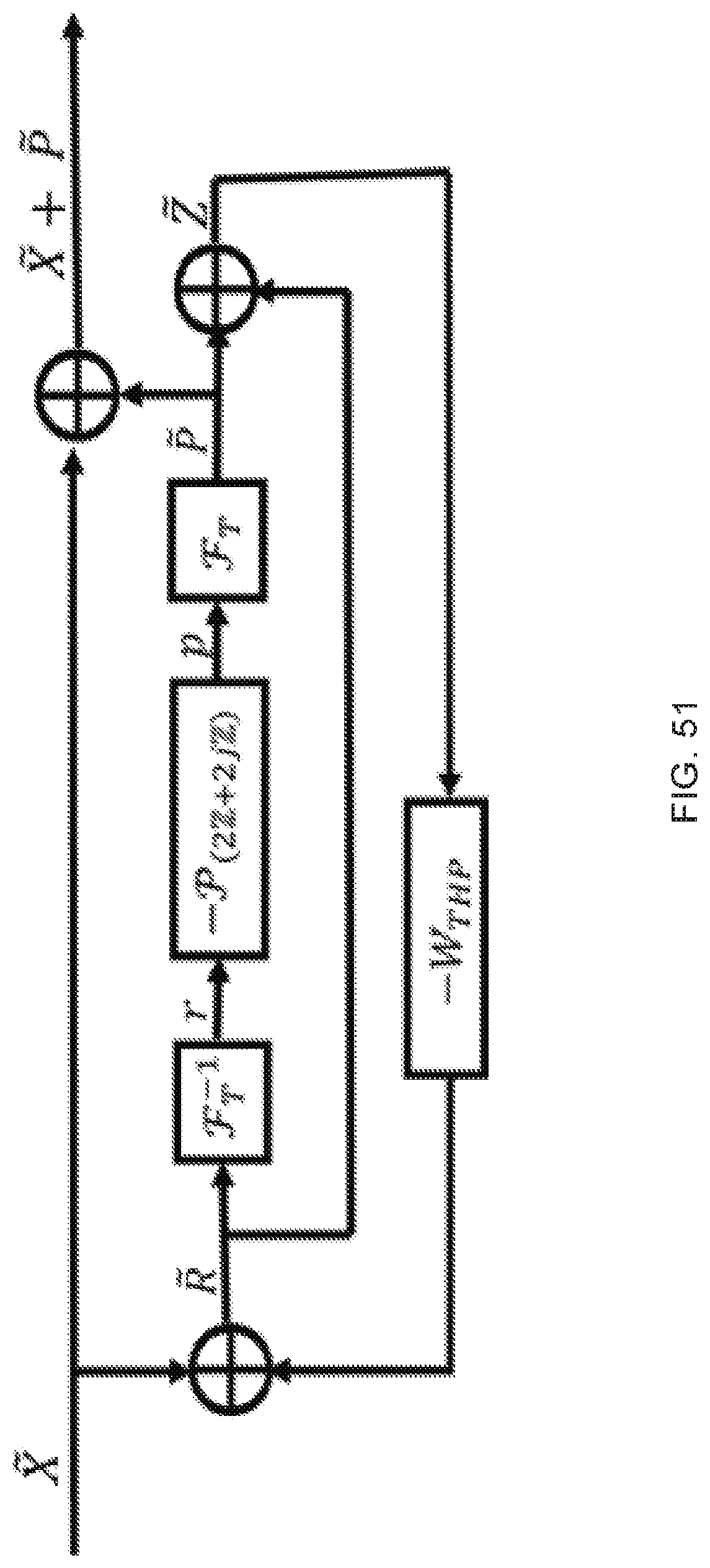
D00059
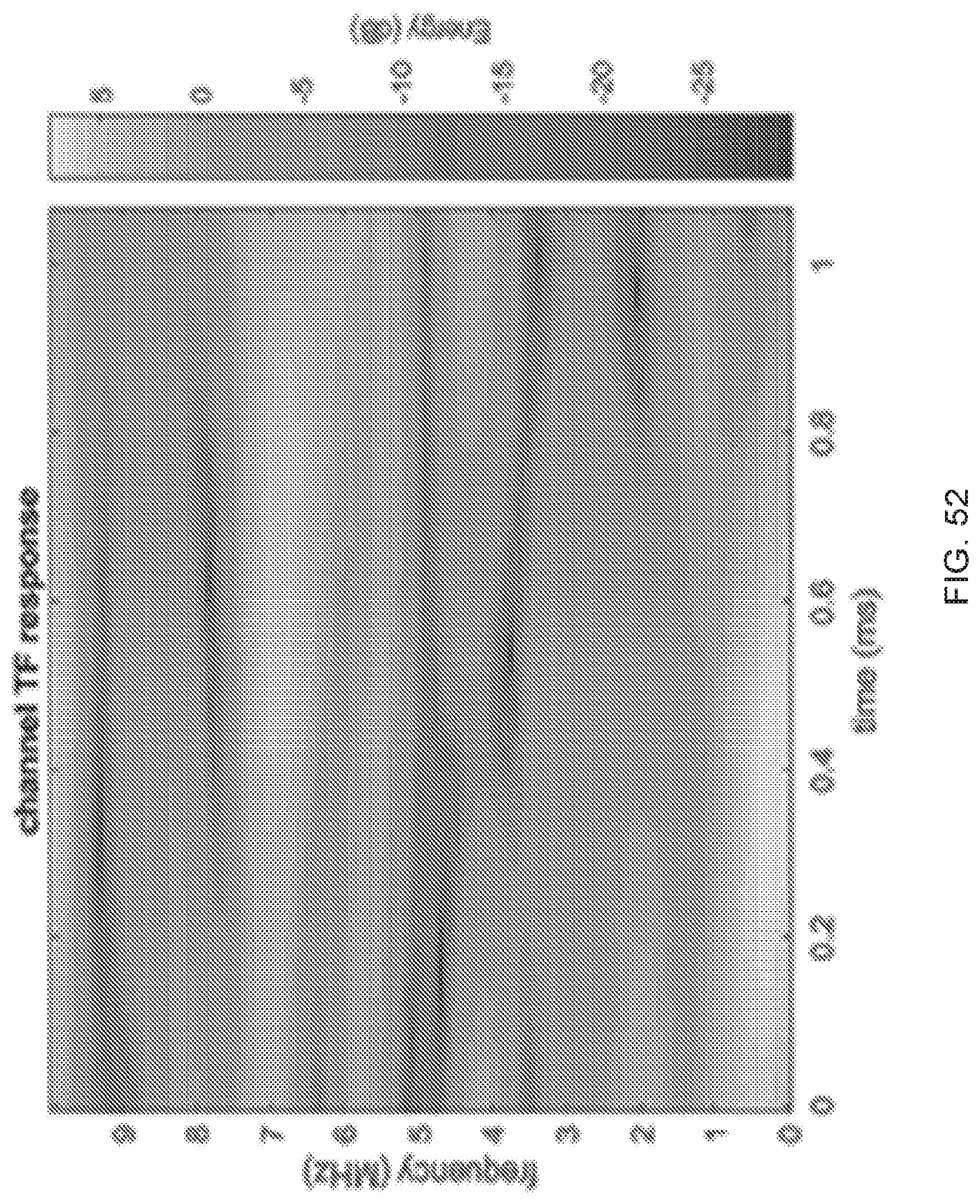
D00060
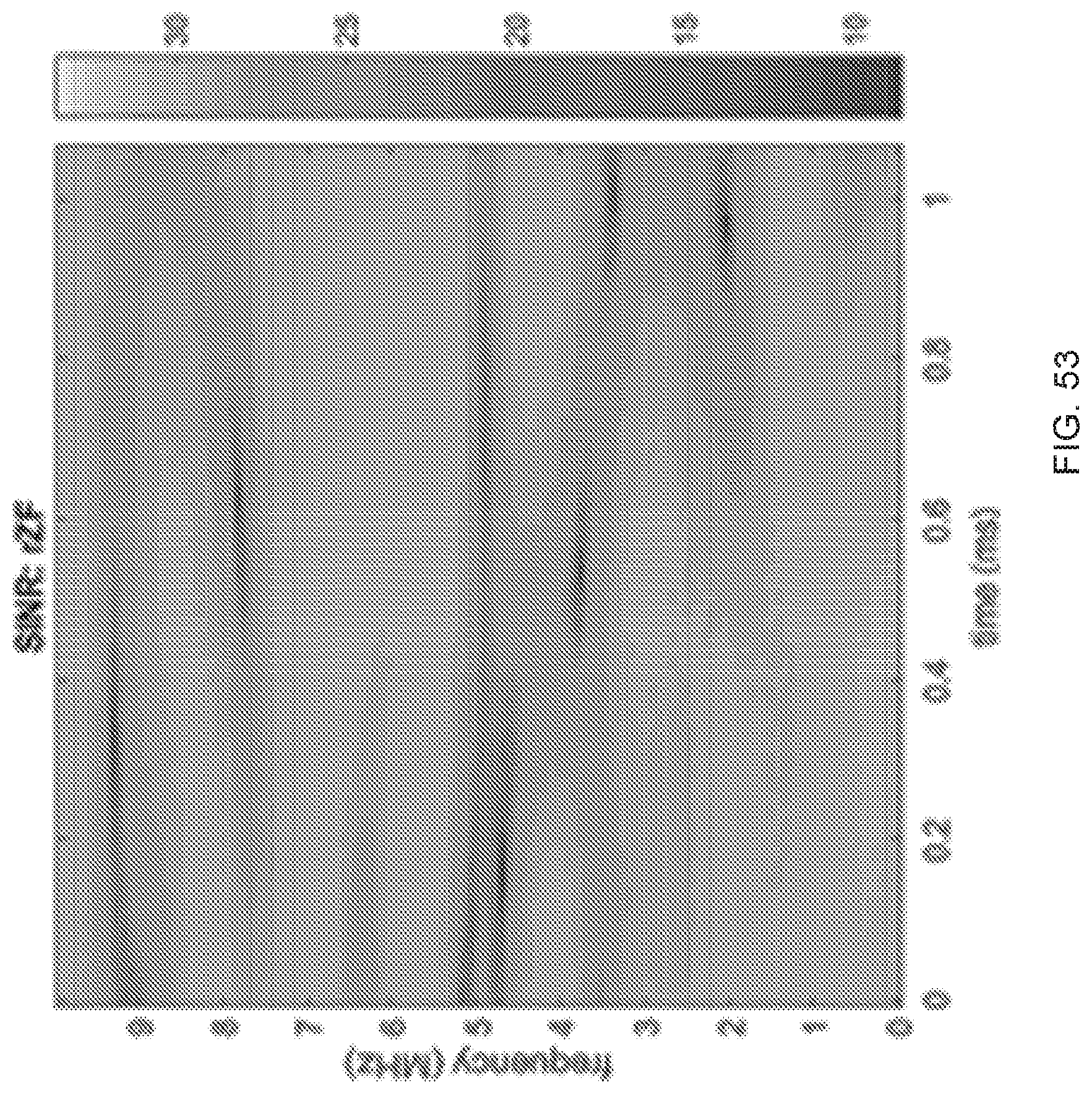
D00061
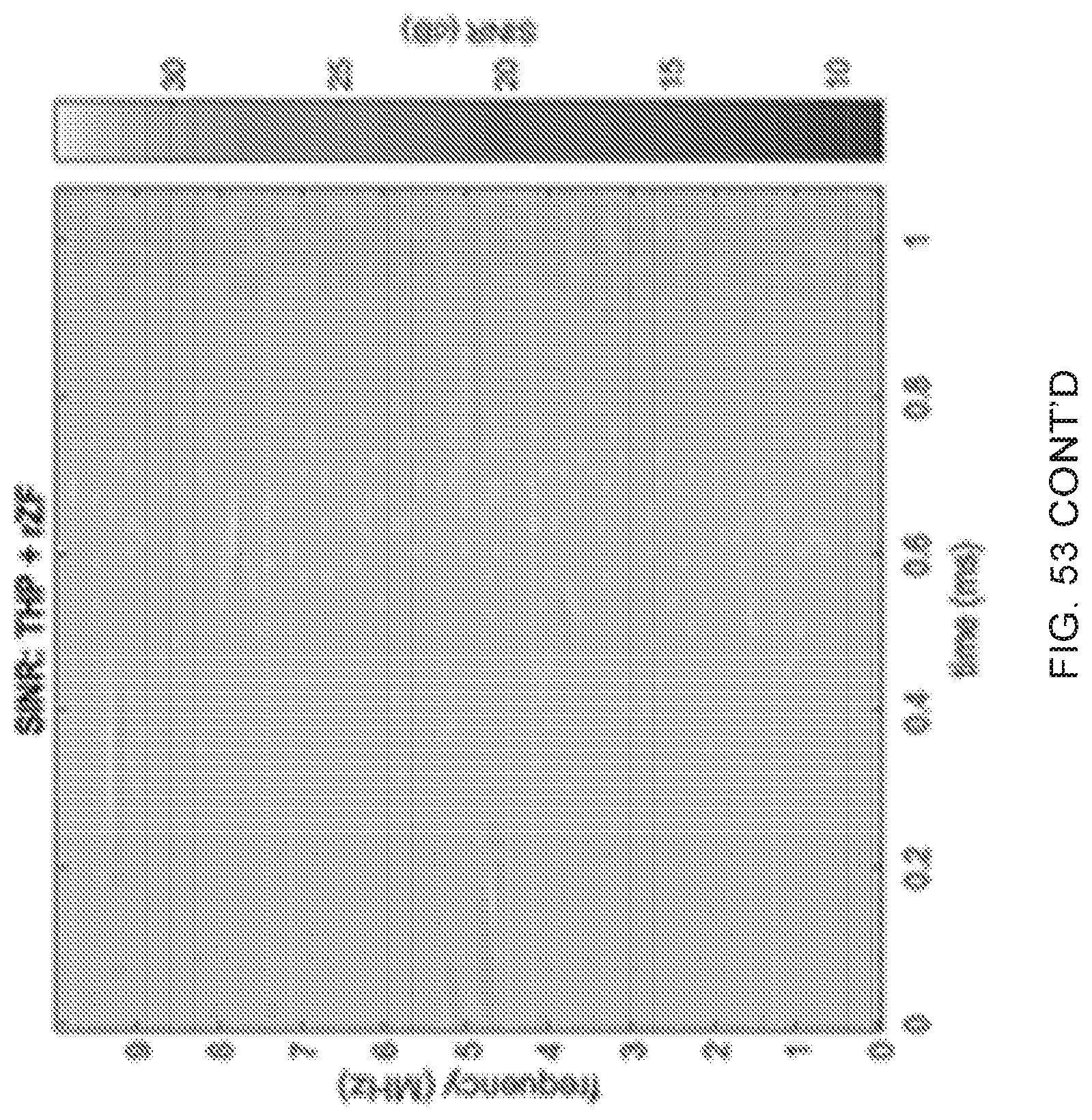
D00062
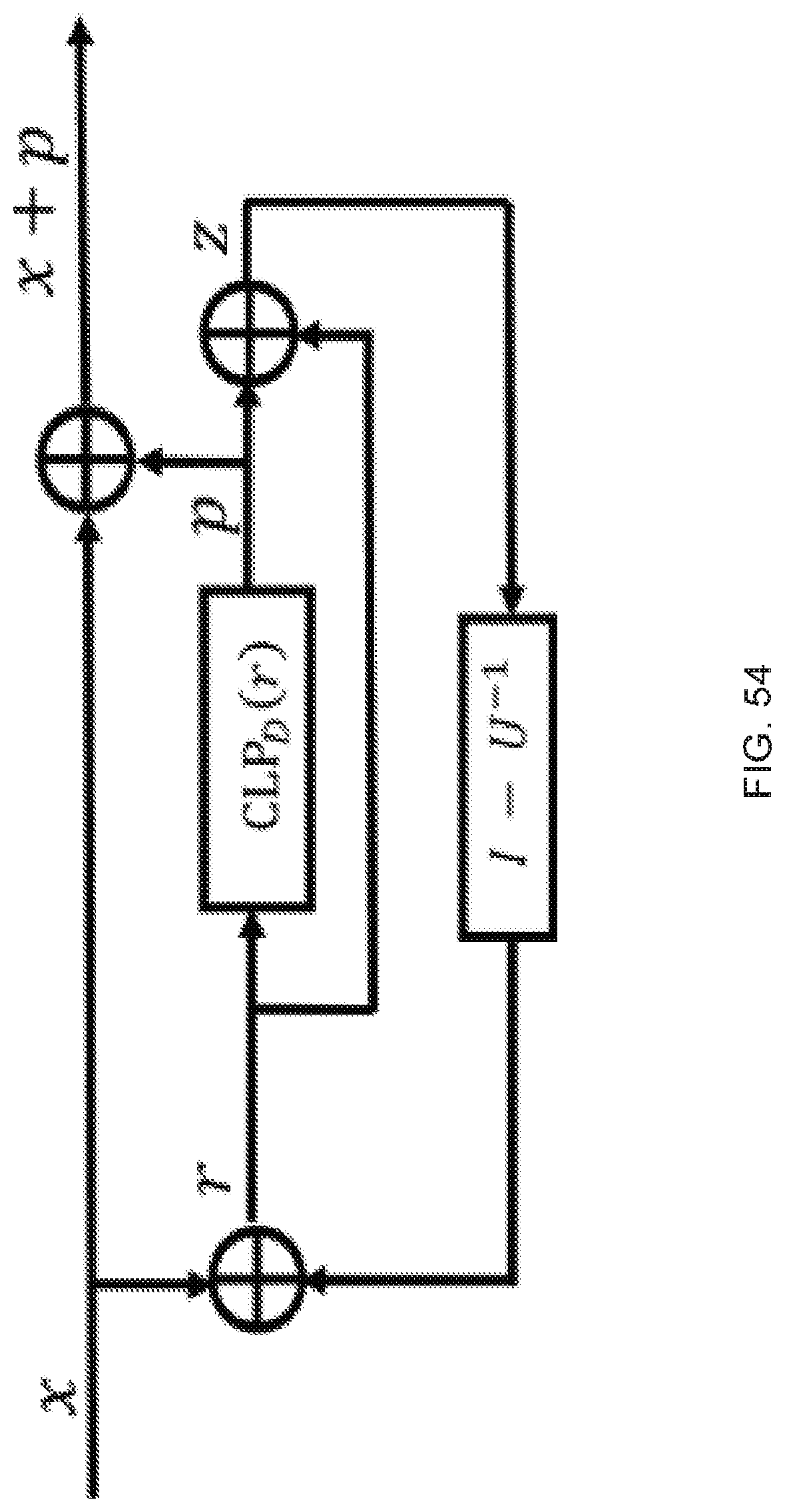
D00063
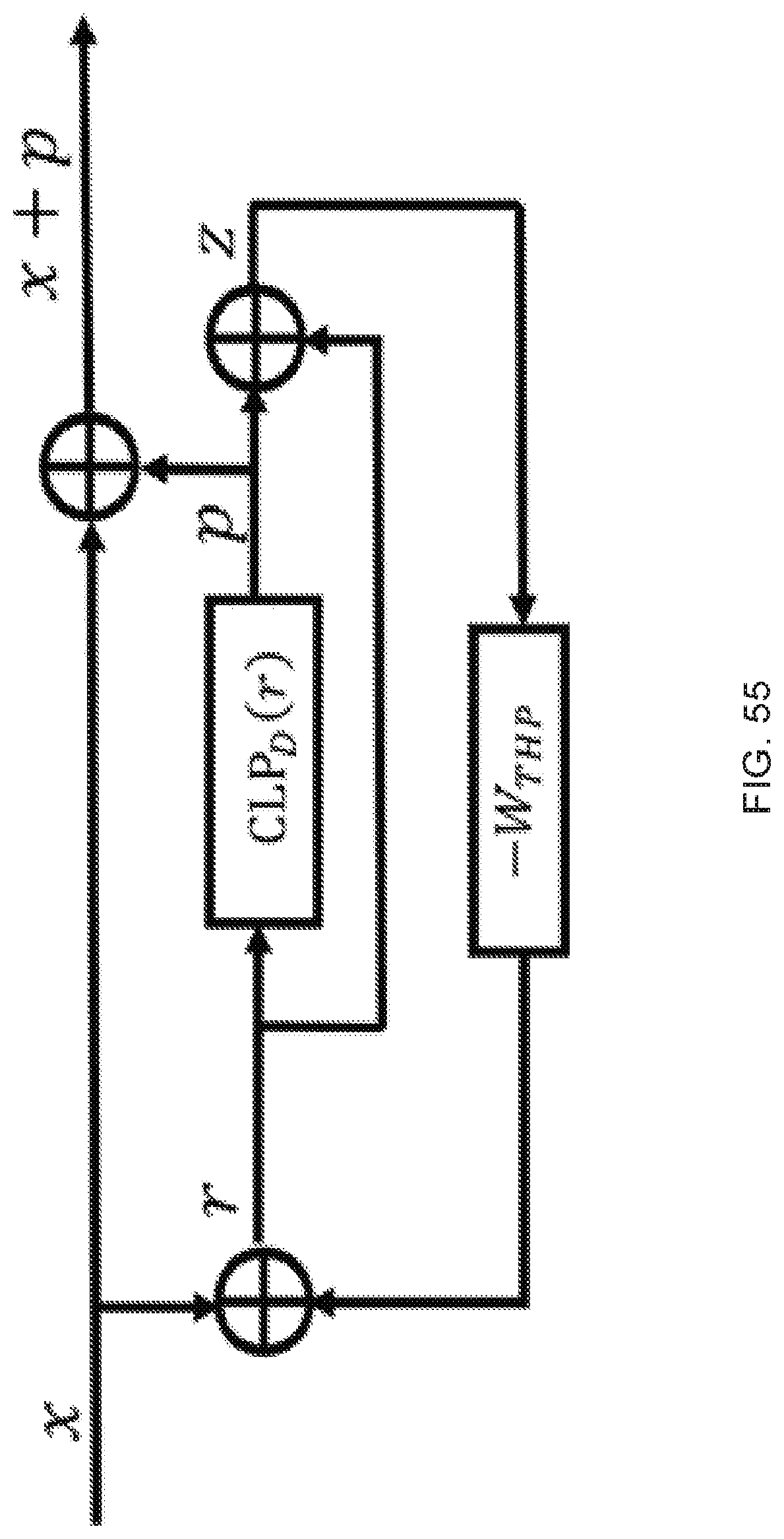
D00064

D00065
D00066
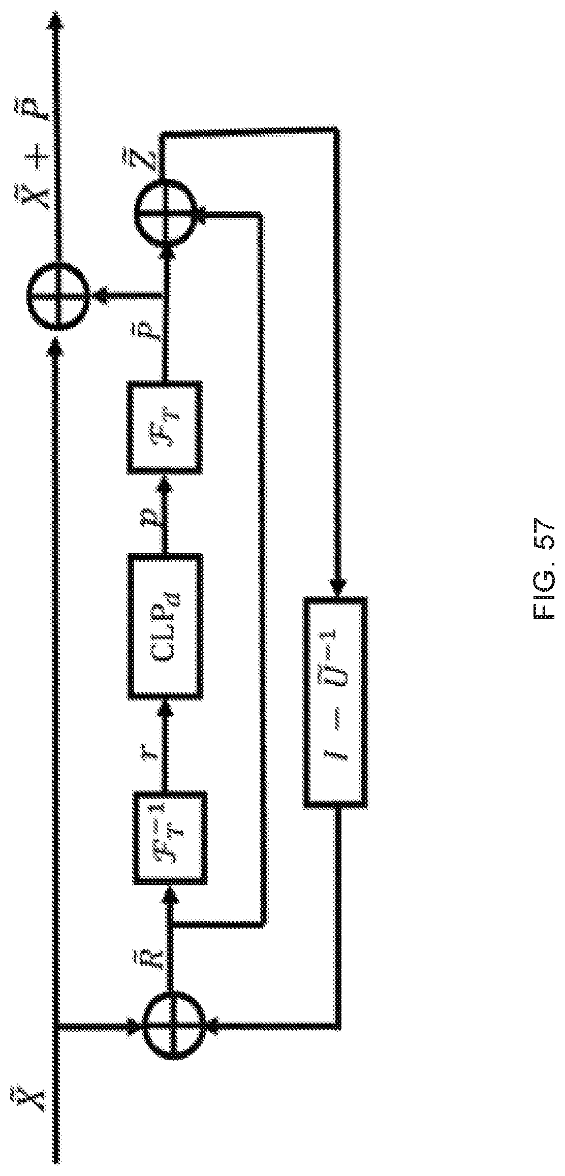
D00067

D00068
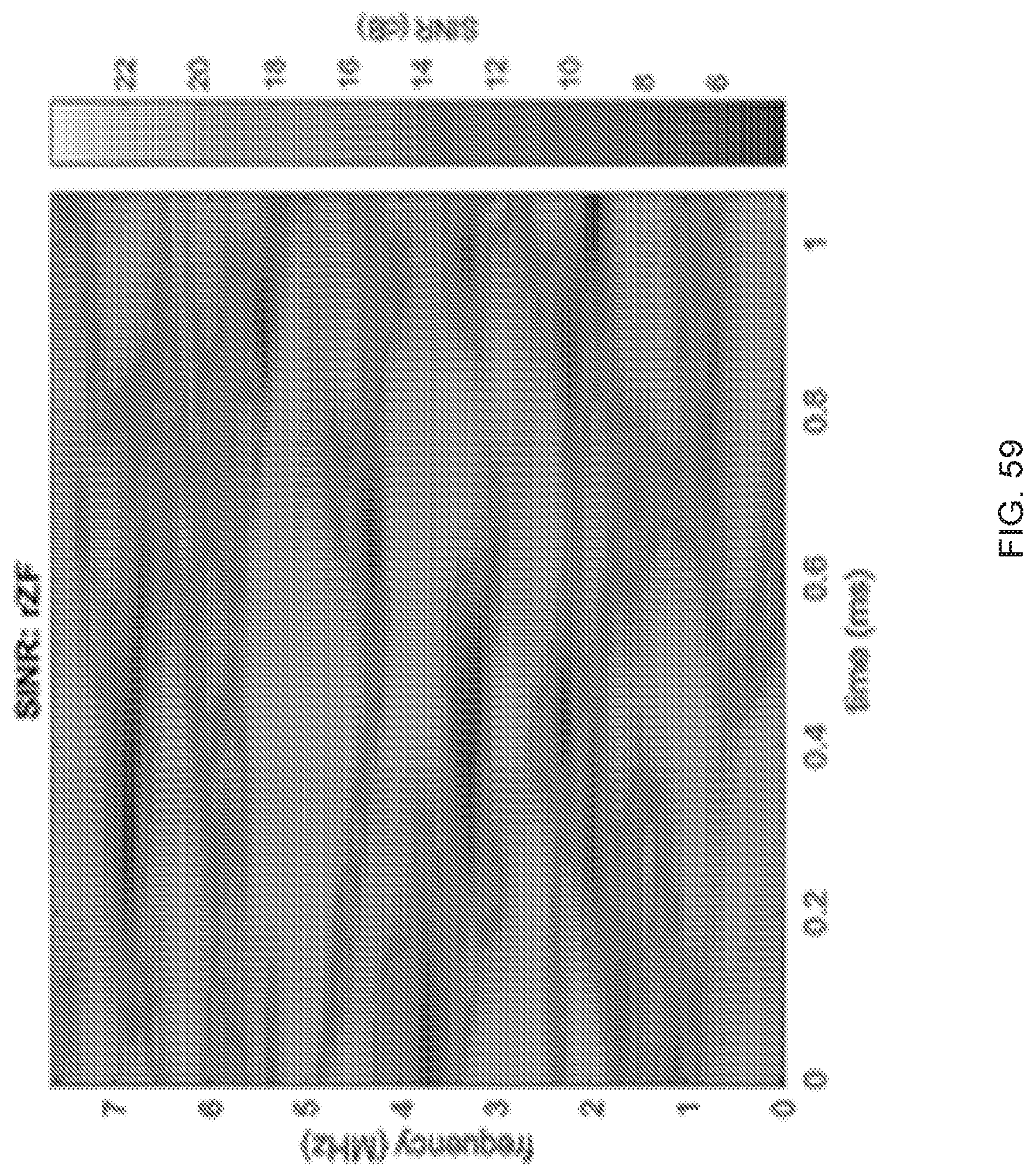
D00069
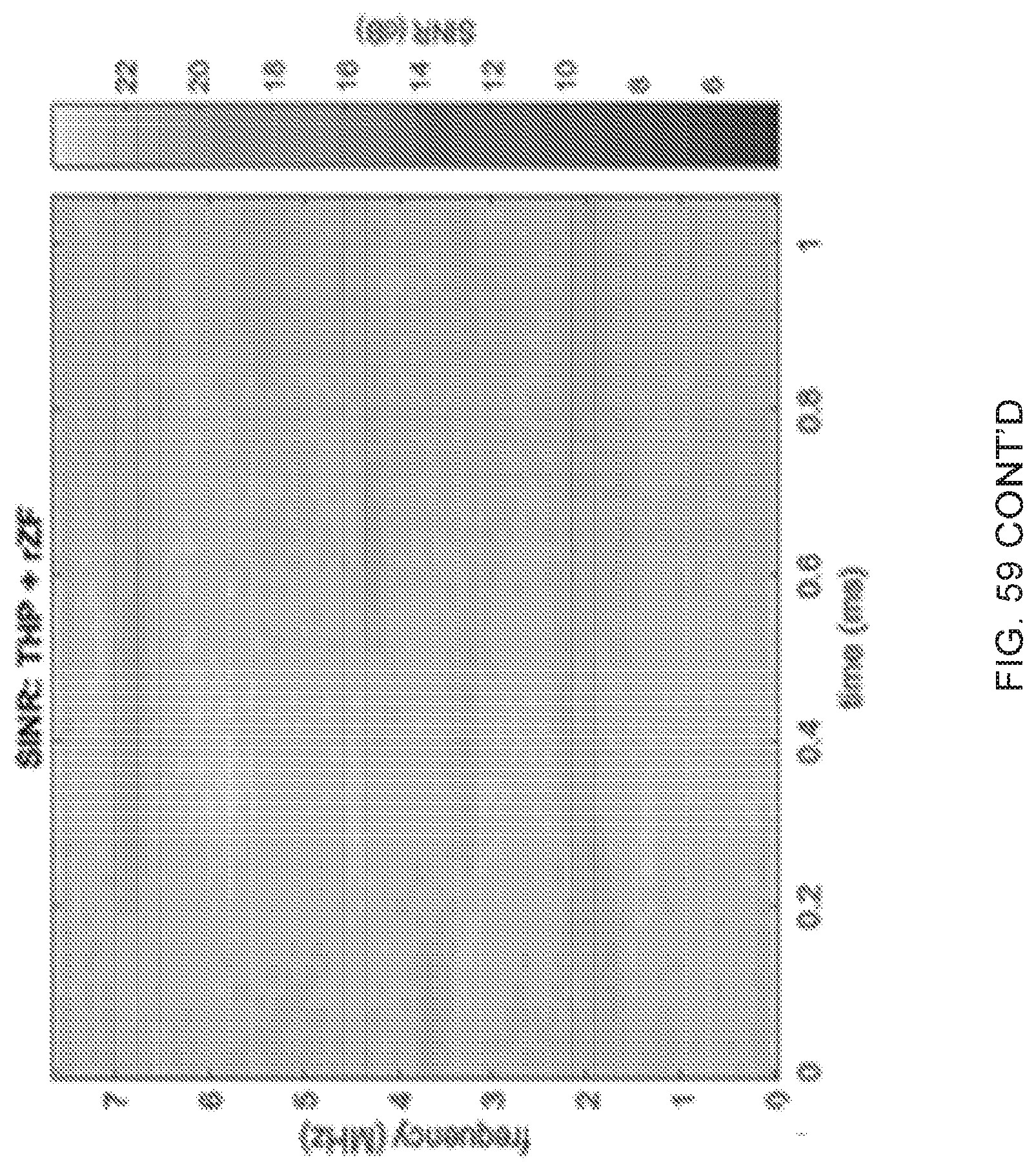
D00070
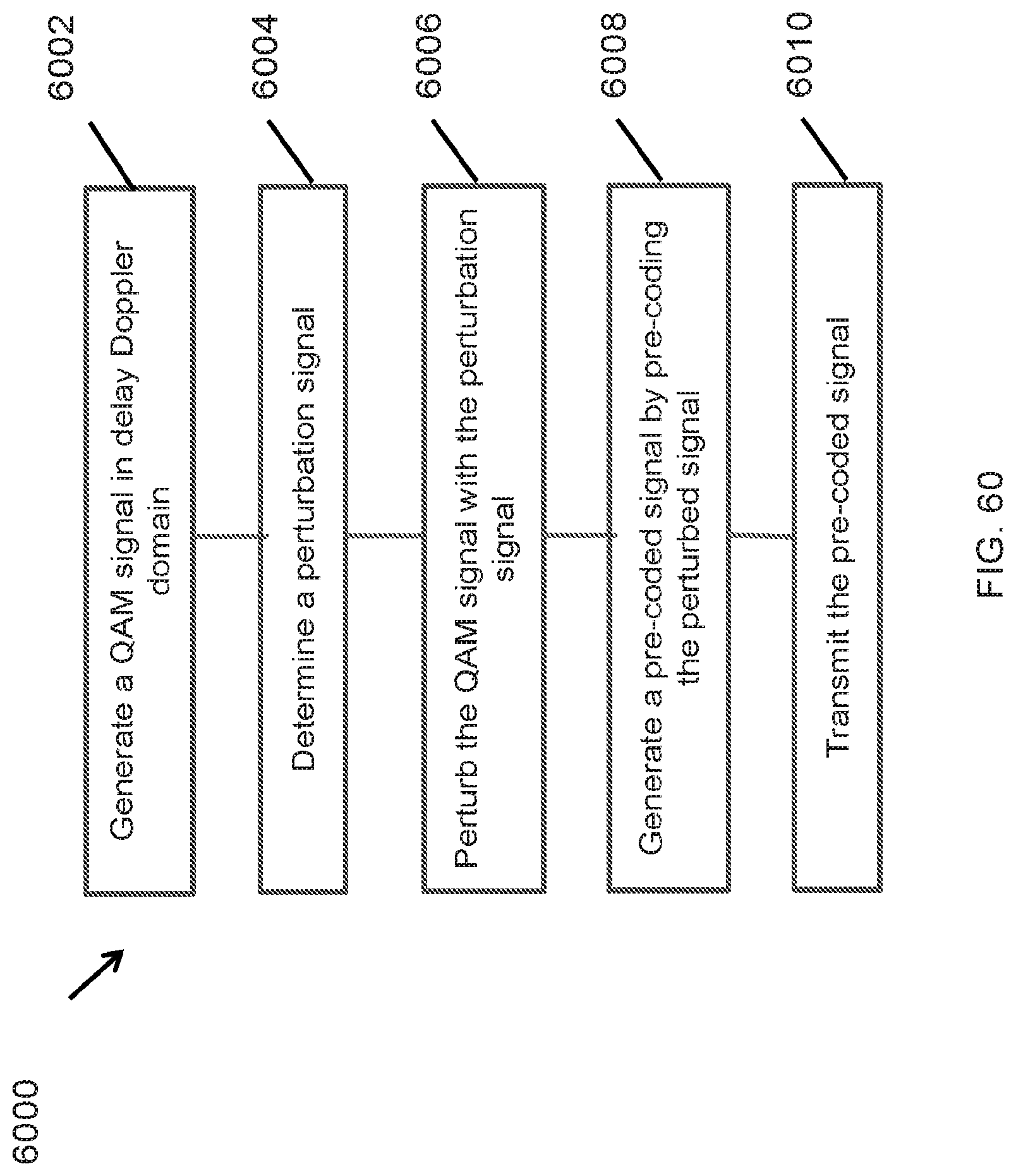
D00071
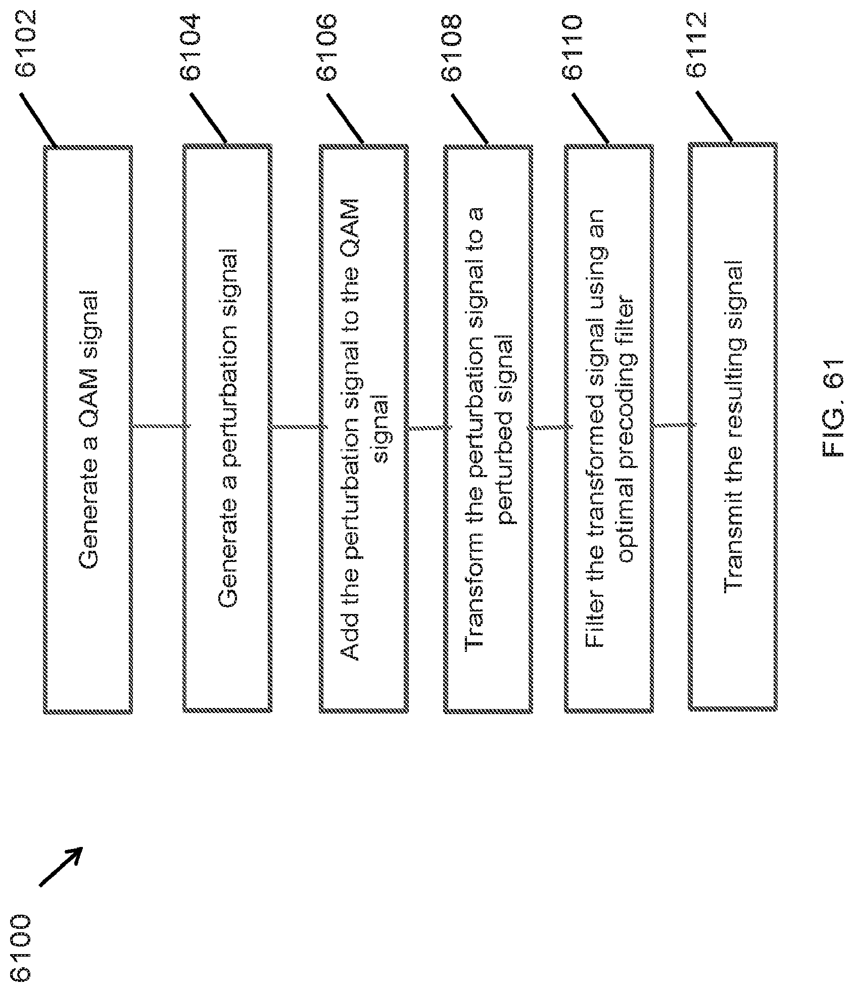
D00072
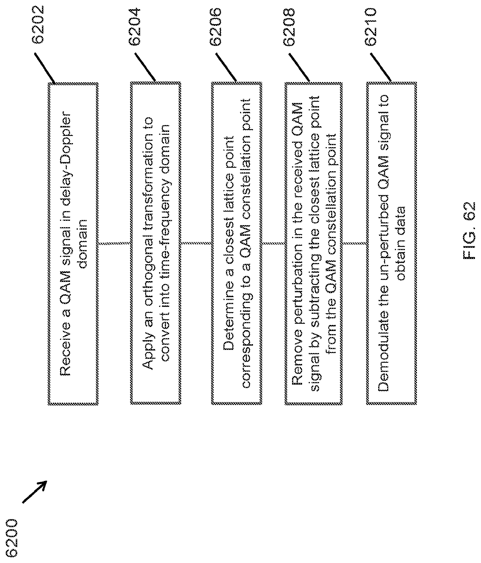
D00073
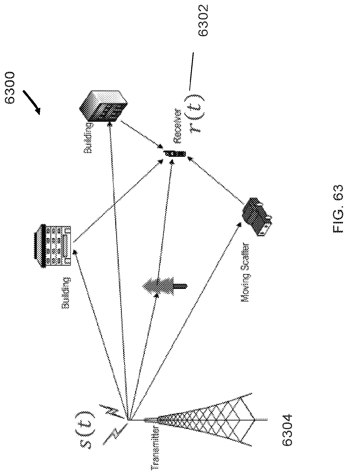
D00074
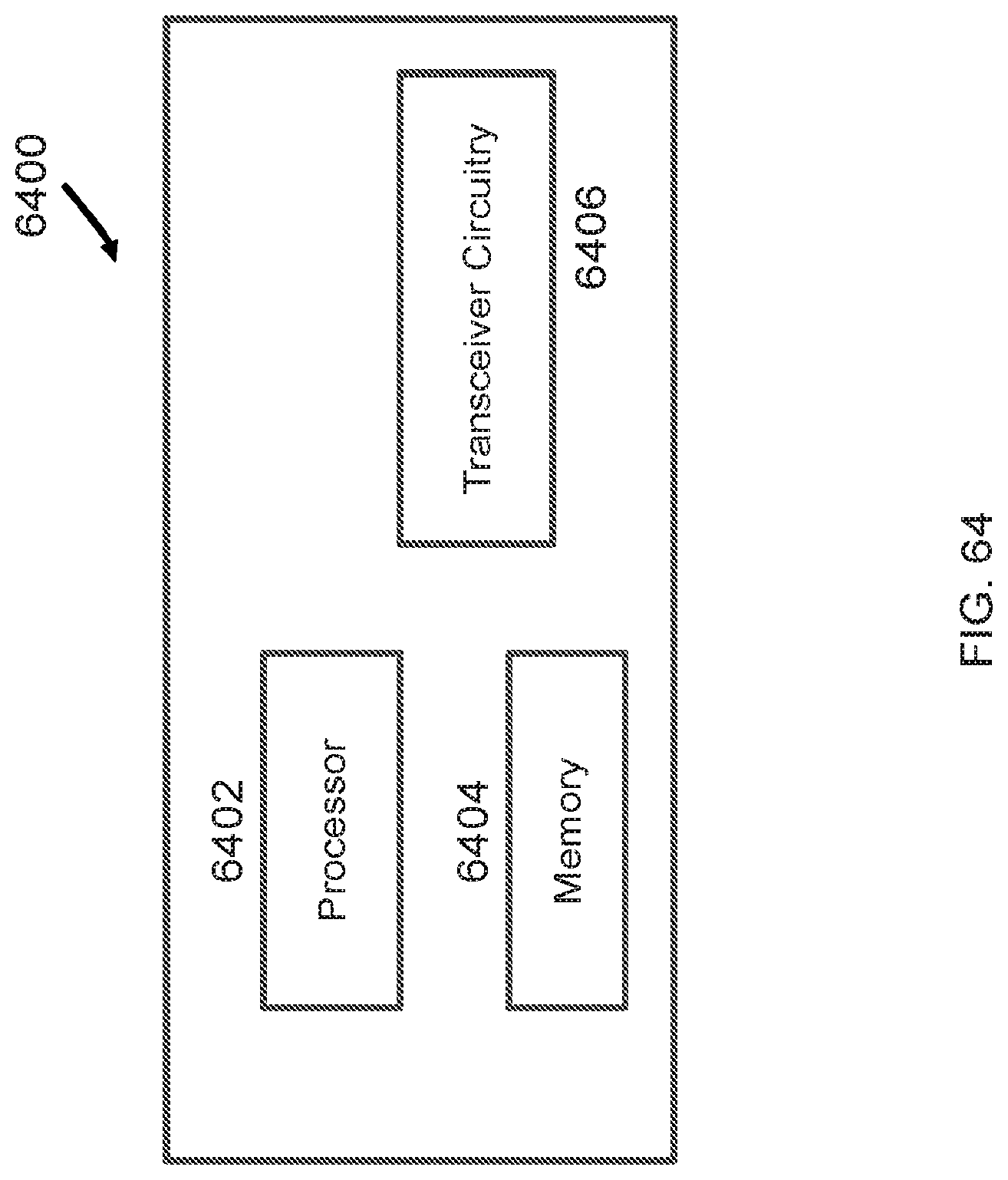
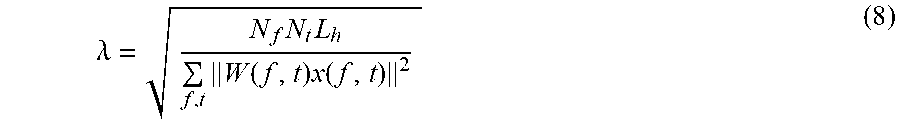


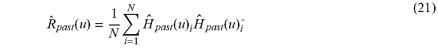


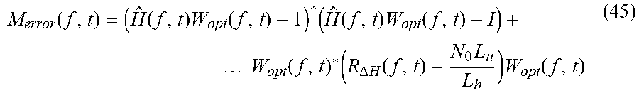


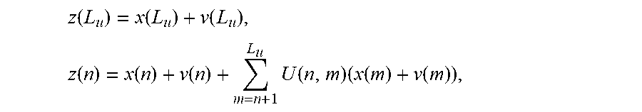
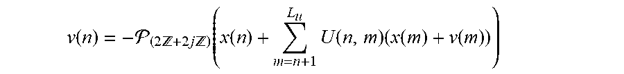
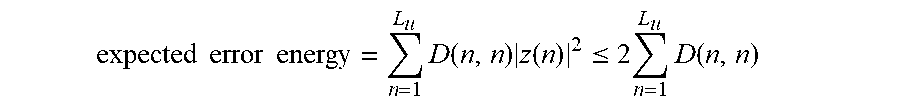


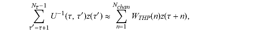
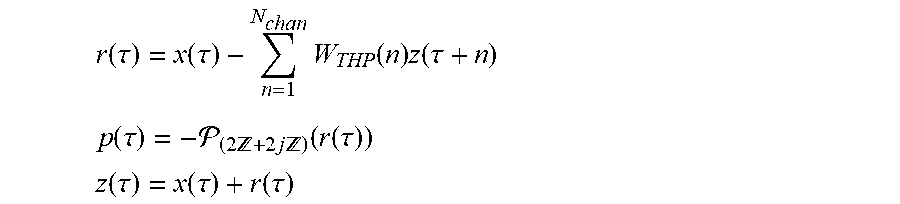

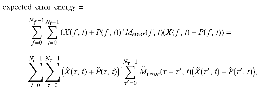
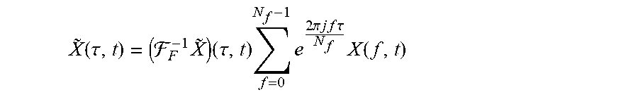

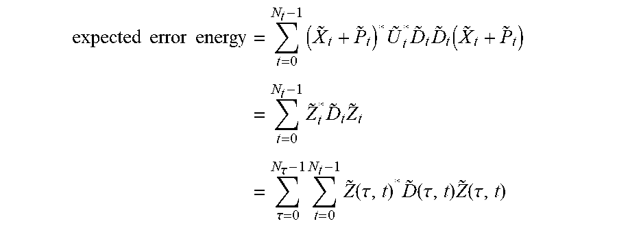

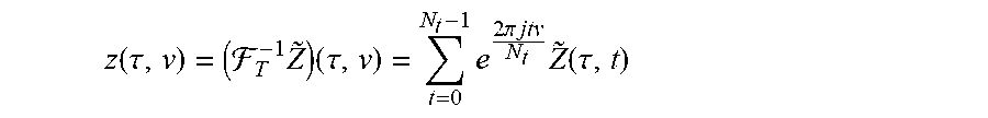
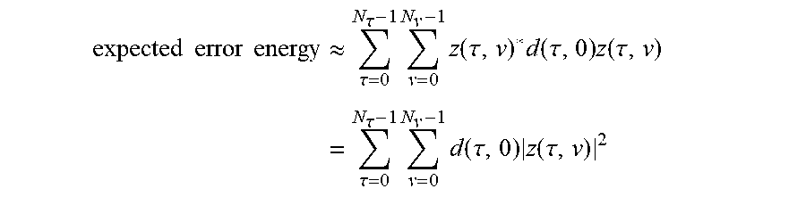
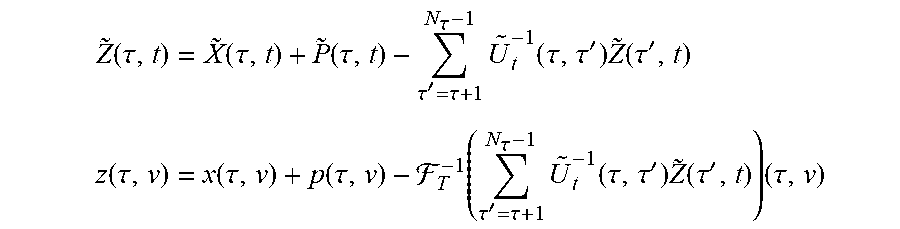
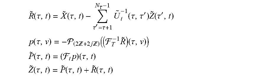
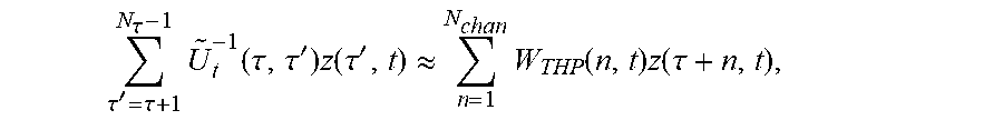
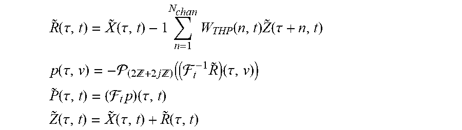
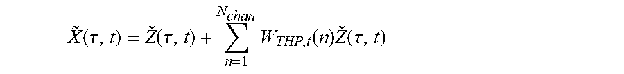
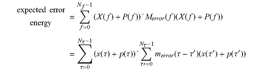

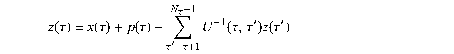


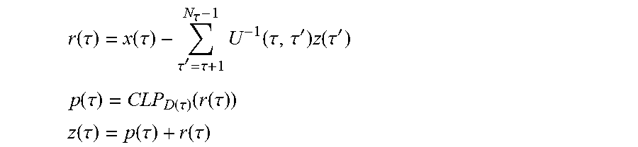
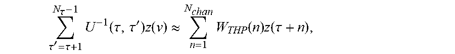
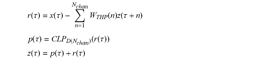
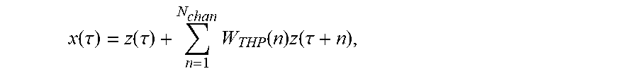
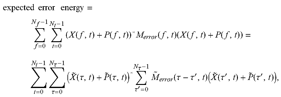
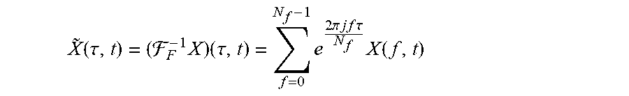

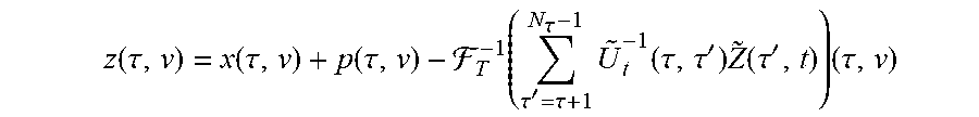
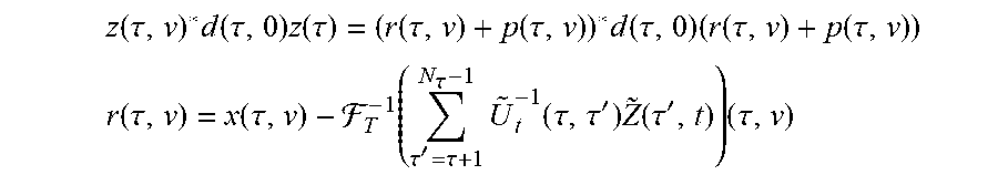

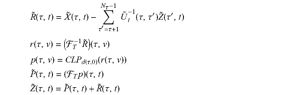
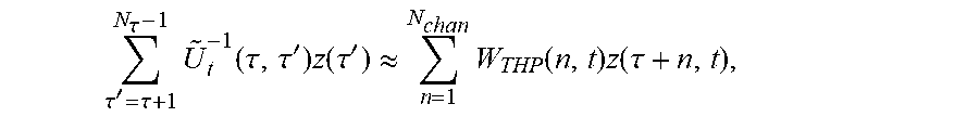
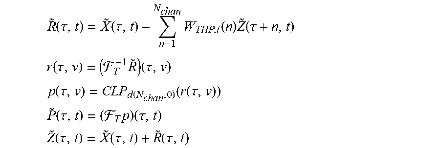

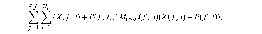


P00001

P00002

P00003

P00004

P00005

P00006

P00007

P00008

P00009

P00010

P00011

XML
uspto.report is an independent third-party trademark research tool that is not affiliated, endorsed, or sponsored by the United States Patent and Trademark Office (USPTO) or any other governmental organization. The information provided by uspto.report is based on publicly available data at the time of writing and is intended for informational purposes only.
While we strive to provide accurate and up-to-date information, we do not guarantee the accuracy, completeness, reliability, or suitability of the information displayed on this site. The use of this site is at your own risk. Any reliance you place on such information is therefore strictly at your own risk.
All official trademark data, including owner information, should be verified by visiting the official USPTO website at www.uspto.gov. This site is not intended to replace professional legal advice and should not be used as a substitute for consulting with a legal professional who is knowledgeable about trademark law.