Systems and Methods for Adaptive EV Charging
Kind Code
U.S. patent application number 16/786803 was filed with the patent office on 2020-08-13 for systems and methods for adaptive ev charging. This patent application is currently assigned to California Institute of Technology. The applicant listed for this patent is California Institute of Technology. Invention is credited to Zachary J. Lee, Tongxin Li, Steven H. Low, Sunash B. Sharma.
| Application Number | 20200254896 16/786803 |
| Document ID | 20200254896 / US20200254896 |
| Family ID | 1000004657005 |
| Filed Date | 2020-08-13 |
| Patent Application | download [pdf] |


View All Diagrams
| United States Patent Application | 20200254896 |
| Kind Code | A1 |
| Lee; Zachary J. ; et al. | August 13, 2020 |
Systems and Methods for Adaptive EV Charging
Abstract
Systems and methods in accordance with embodiments of the invention impalement adaptive electric vehicle (EV) charging. One embodiment includes one or more electric vehicle supply equipment (EVSE); an adaptive EV charging platform, including a processor; a memory containing: an adaptive EV charging application; a plurality of EV charging parameters. In addition, the processor is configured by the adaptive EV charging application to: collect the plurality of EV charging parameters from one or more EVSEs, simulate EV charging control routines and push out updated EV charging control routines to the one or more EVSEs. Additionally, the adaptive EV charging platform is configured to control charging of EVs based upon the plurality of EV charging parameters collected from at least one EVSE.
| Inventors: | Lee; Zachary J.; (Pasadena, CA) ; Li; Tongxin; (Pasadena, CA) ; Low; Steven H.; (La Canada, CA) ; Sharma; Sunash B.; (Pasadena, CA) | ||||||||||
| Applicant: |
|
||||||||||
|---|---|---|---|---|---|---|---|---|---|---|---|
| Assignee: | California Institute of
Technology Pasadena CA |
||||||||||
| Family ID: | 1000004657005 | ||||||||||
| Appl. No.: | 16/786803 | ||||||||||
| Filed: | February 10, 2020 |
Related U.S. Patent Documents
| Application Number | Filing Date | Patent Number | ||
|---|---|---|---|---|
| 62803157 | Feb 8, 2019 | |||
| 62964504 | Jan 22, 2020 | |||
| Current U.S. Class: | 1/1 |
| Current CPC Class: | B60L 53/51 20190201; B60L 53/62 20190201; B60L 53/64 20190201; B60L 53/63 20190201 |
| International Class: | B60L 53/62 20060101 B60L053/62; B60L 53/63 20060101 B60L053/63; B60L 53/51 20060101 B60L053/51; B60L 53/64 20060101 B60L053/64 |
Goverment Interests
STATEMENT OF FEDERALLY SPONSORED RESEARCH
[0002] This invention was made with government support under Grant No. CCF1637598 awarded by the National Science Foundation. The government has certain rights in the invention.
Claims
1. An adaptive electric vehicle charging system, comprising: one or more electric vehicle supply equipment (EVSE): an adaptive electric vehicle (EVT) charging platform, comprising: a processor; a memory containing: an adaptive EV charging application; a plurality of EV charging parameters; wherein the processor is configured by the adaptive EV charging application to: collect the plurality of EV charging parameters from one or more EVSEs, simulate EV charging control routines and push out updated EV charging control routines to the one or more EVSEs; and wherein the adaptive EV charging platform is configured to control charging of EVs based upon the plurality of EV charging parameters collected from at least one EVSE.
2. The adaptive electric vehicle charging system of claim 1, wherein the processor is configured to learn an underlying distribution of EV arrival time, session duration, and energy delivered.
3. The adaptive electric vehicle charging system of claim 1, wherein the processor is configured to learn an underlying distribution of EV arrival time, session duration, and energy delivered using Gaussian mixture models (GMMs).
4. The adaptive electric vehicle charging system of claim 3, wherein the GMMs are used to predict EV users' charging behavior.
5. The adaptive electric vehicle charging system of claim 3, wherein the processor is further configured to use the GMMs to control charging of large numbers of EVs in order to smooth a difference in electricity demand and amount of available solar energy throughout the day (Duck curve).
6. The adaptive electric vehicle charging system of claim 3, wherein the processor is further configured to train the GMMs based on a training dataset and predict a charging duration and energy delivered.
7. The adaptive electric vehicle charging system of claim 3, wherein the GMMs are population-level GMMs (P-GMM).
8. The adaptive electric vehicle charging system of claim 3, wherein the GMMs are individual-level GMMs (I-GMM).
9. The adaptive electric vehicle charging system of claim 1, further comprising a power distribution network.
10. The adaptive electric vehicle charging system of claim 1, wherein the plurality of EV charging parameters comprises EV driver laxity data.
11. The adaptive electric vehicle charging system of claim 1, wherein the processor is further configured by the adaptive EV charging application to: receive an EV request for charging, determine an amount of energy and a duration for delivering the amount of energy to the EV, optimize time-varying charging rate based on time of day and electric system load, and synchronize with one or more EVSEs to deliver optimum charge to the EV.
12. An adaptive electric vehicle charging platform, comprising: a processor; a memory containing: an adaptive EV charging application; a plurality of EV charging parameters; wherein the processor is configured by the adaptive EV charging application to: collect the plurality of EV charging parameters from one or more EVSEs, simulate EV charging control routines and push out updated EV charging control routines to the one or more EVSEs; and wherein the processor is configured by the adaptive EV charging application to: receive an EV request for charging, determine an amount of energy and a duration for delivering the amount of energy to the EV, optimize time-varying charging rate based on time of day and electric system load, and synchronize with an electric vehicle charging station to deliver optimum charge to the EV.
13. The adaptive electric vehicle charging platform of claim 12, wherein the processor is configured to learn an underlying distribution of EV arrival time, session duration, and energy delivered.
14. The adaptive electric vehicle charging platform of claim 12, wherein the processor is configured to learn an underlying distribution of EV arrival time, session duration, and energy delivered using Gaussian mixture models (GMMs).
15. The adaptive electric vehicle charging platform of claim 14, wherein the GMMs are used to predict EV users' charging behavior.
16. The adaptive electric vehicle charging platform of claim 14, wherein the processor is further configured to train the GMMs based on a training dataset and predict a charging duration and energy delivered.
17. The adaptive electric vehicle charging platform of claim 12, wherein the processor is further configured to learn an underlying model of an electric vehicle's battery charging behavior.
18. The adaptive electric vehicle charging platform of claim 12, wherein the processor is further configured to learn battery models based on a training dataset, and to predict a maximum charging rate and threshold state of charge for a linear 2-stage battery model.
19. The adaptive electric vehicle charging platform of claim 12, wherein the processor is further configured to use learned battery models to simulate EV charging control routines.
20. The adaptive electric vehicle charging platform of claim 12, wherein the processor is further configured to use learned battery models to predict energy delivered.
Description
CROSS-REFERENCE TO RELATED APPLICATIONS
[0001] The present invention claims priority to U.S. Provisional Patent Application Ser. No. 62/803,157 entitled "Date-Driven Approach To Joint EV And Solar Optimization Using Predictions" to Zachary J. Lee et. al., filed Feb. 8, 2019, and to U.S. Provisional Patent Application Ser. No. 62/964,504 entitled "EV Charging Optimization Using Adaptive Charging Network Data" to Zachary J. Lee et. al., filed Jan. 22, 2020, the disclosures of which are herein incorporated by reference in their entirety.
FIELD OF THE INVENTION
[0003] The present invention generally relates to electric vehicles and more specifically relates to systems and methods for adaptive electric vehicle charging.
BACKGROUND
[0004] An incredible amount of infrastructure is relied upon to transport electricity from power stations, where the majority of electricity is currently generated, to where it is consumed by individuals. Power stations can generate electricity in a number of ways including using fossil fuels or using renewable energy sources such as solar, wind, and hydroelectric sources. Substations typically do not generate electricity, but can change the voltage level of the electricity as well as provide protection to other grid infrastructure during faults and outages. From here, the electricity travels over distribution lines to bring electricity to locations where it is consumed such as homes, businesses, and schools. The term "smart grid" describes a new approach to power distribution which leverages advanced technology to track and manage the distribution of electricity. A smart grid applies upgrades to existing power grid infrastructure including the addition of more renewable energy sources, advanced smart meters that digitally record power usage in real time, and bidirectional energy flow that enables the generation and storage of energy in additional places along the electric grid.
[0005] Electric vehicles (EVs), which include plug-in hybrid electric vehicles (PHEVs), can use an electric motor for propulsion. EV adoption has been spurred by federal, state, and local government policies providing various incentives (e.g. rebates, fast lanes, parking, etc.). Continued EV adoption is likely to have a significant, impact on the future smart grid due to the additional stress load that EVs add to the grid (an EV's power demand can be many times that of an average residential house).
[0006] Duck curve, named after its resemblance to a duck, shows a difference in electricity demand and amount of available solar energy throughout the day. When the sun is shining, solar floods the market and then drops off as electricity demand peaks in the evening.
SUMMARY OF THE INVENTION
[0007] Systems and methods in accordance with embodiments of the invention impalement adaptive electric vehicle (EV) charging. One embodiment includes one or more electric vehicle supply equipment (EVSE); an adaptive EV charging platform, including a processor; a memory containing: an adaptive EV charging application: a plurality of EV charging parameters. In addition, the processor is configured by the adaptive EV charging application to: collect the plurality of EV charging parameters from one or more EVSEs, simulate EV charging control routines and push out updated EV charging control routines to the one or more EVSEs. Additionally, the adaptive EV charging platform is configured to control charging of EVs based upon the plurality of EV charging parameters collected from at least one EVSE.
[0008] In a further embodiment, the processor is configured to learn an underlying distribution of EV arrival time, session duration, and energy delivered.
[0009] In still a further embodiment, the processor is configured to learn an underlying distribution of EV arrival time, session duration, and energy delivered using Gaussian mixture models (GMMs).
[0010] In a yet further embodiment, the GMMs are used to predict EV users' charging behavior.
[0011] In a yet further embodiment again, the processor is further configured to use the GMMs to control charging of large numbers of EVs in order to smooth a difference in electricity demand and amount of available solar energy throughout the day (Duck curve).
[0012] In another embodiment again, the processor is further configured to train the GMMs based on a training dataset and predict a charging duration and energy delivered.
[0013] In a yet further embodiment, the GMMs are population-level GMMs (P-GMM).
[0014] In another embodiment again, the GMMs are individual-level GMMs (I-GMM).
[0015] In another embodiment still, the adaptive EV charging system further includes a power distribution network.
[0016] In still a further embodiment, the plurality of EV charging parameters include EV driver laxity data.
[0017] In another embodiment still, the processor is further configured by the adaptive EV charging application to: receive an EV request for charging, determine an amount of energy and a duration for delivering the amount of energy to the EV, optimize time-varying charging rate based on time of day and electric system load, and synchronize with one or more EVSEs to deliver optimum charge to the EV.
[0018] In a further additional embodiment, an adaptive electric vehicle charging platform includes: a processor; a memory containing: an adaptive EV charging application; a plurality of EV charging parameters; wherein the processor is configured by the adaptive EV charging application to: collect the plurality of EV charging parameters from one or more EVSEs, simulate EV charging control routines and push out updated EV charging control routines to the one or more EVSEs; and wherein the processor is configured by the adaptive EV charging application to: receive an EV request for charging, determine an amount of energy and a duration for delivering the amount of energy to the EV, optimize time-varying charging rate based on time of day and electric system load, and synchronize with an electric vehicle charging station to deliver optimum charge to the EV.
[0019] In still yet an other embodiment again, the processor is further configured to learn an underlying model of an electric vehicle's battery charging behavior.
[0020] In a further additional embodiment, the processor is further configured to learn battery models based on a training dataset, and to predict a maximum charging rate and threshold state of charge for a linear 2-stage battery model.
[0021] In still a further additional embodiment, the processor is further configured to use learned battery models to simulate EV charging control routines.
[0022] In still yet another embodiment again, the processor is further configured to use learned battery models to predict energy delivered.
BRIEF DESCRIPTION OF THE DRAWINGS
[0023] FIG. 1 is a diagram conceptually illustrating a power distribution network in accordance with an embodiment of the invention.
[0024] FIG. 2 illustrates adaptive charging network (ACN) data collection from an EV charging site in order to simulate EV charging control routines which are located in a network cloud, and push-out of updated EV charging control routines to the EV charging site in accordance with an embodiment of the invention.
[0025] FIG. 3 illustrate ACN data collection, simulating control routines, and pushing out updated control routines in accordance with an embodiment of the invention.
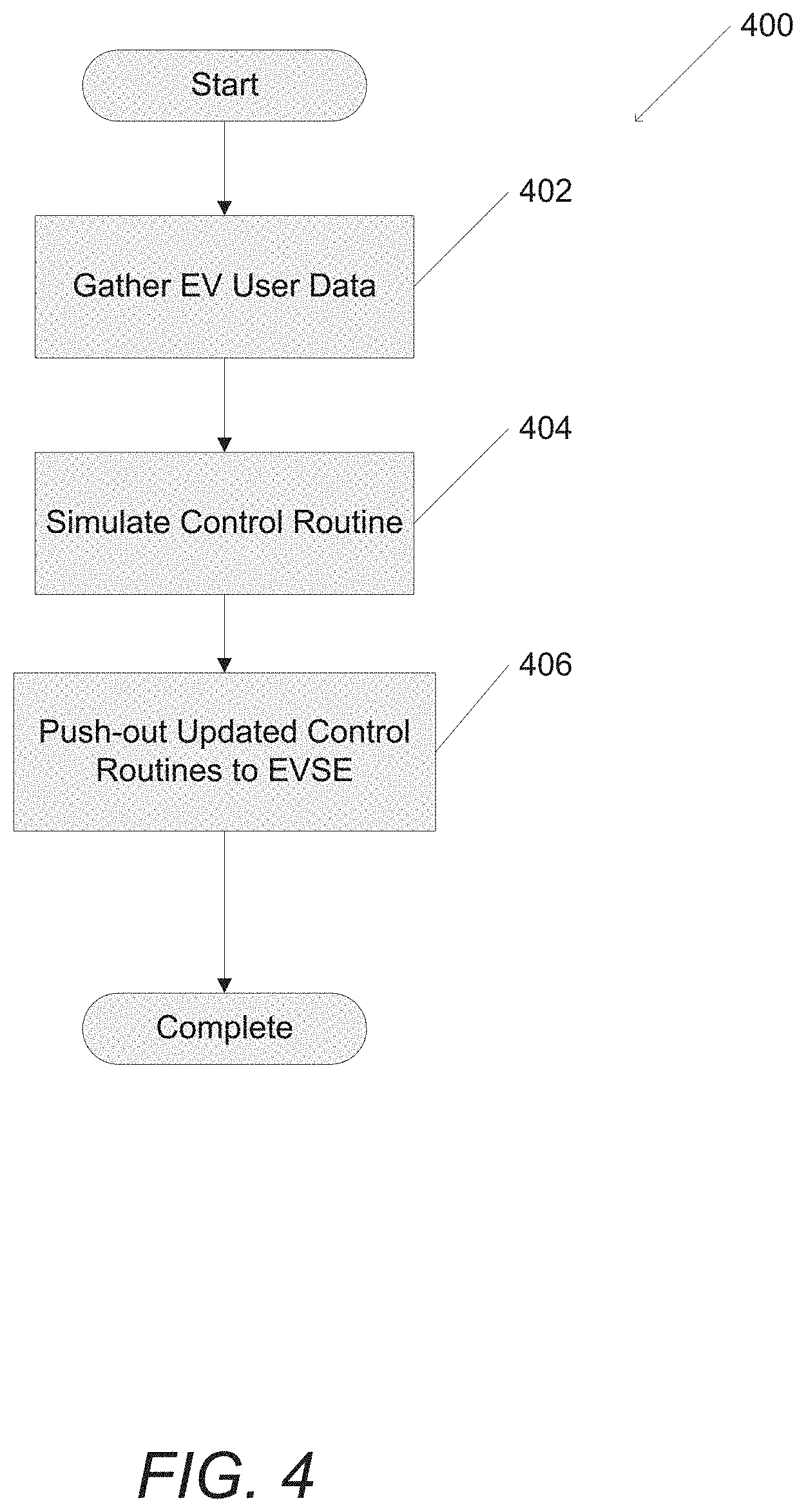
[0026] FIG. 4 is a flow chart illustrating a process for gathering EV user data, simulating control routines, and pushing out updated control routines in accordance with an embodiment of the invention.
[0027] FIG. 5 is a flow chart illustrating a process for receiving an EV user request for charging and delivering optimum charge to the EV user in accordance with an embodiment of the invention.
[0028] FIGS. 6A and 68 illustrate that EV driver laxity can be used to oversubscribe electric vehicle supply equipment in accordance with an embodiment of the invention.
[0029] FIG. 7 illustrates an increase in an amount of demand met using adaptive charging compared to other methods of charging in accordance with an embodiment of the invention.
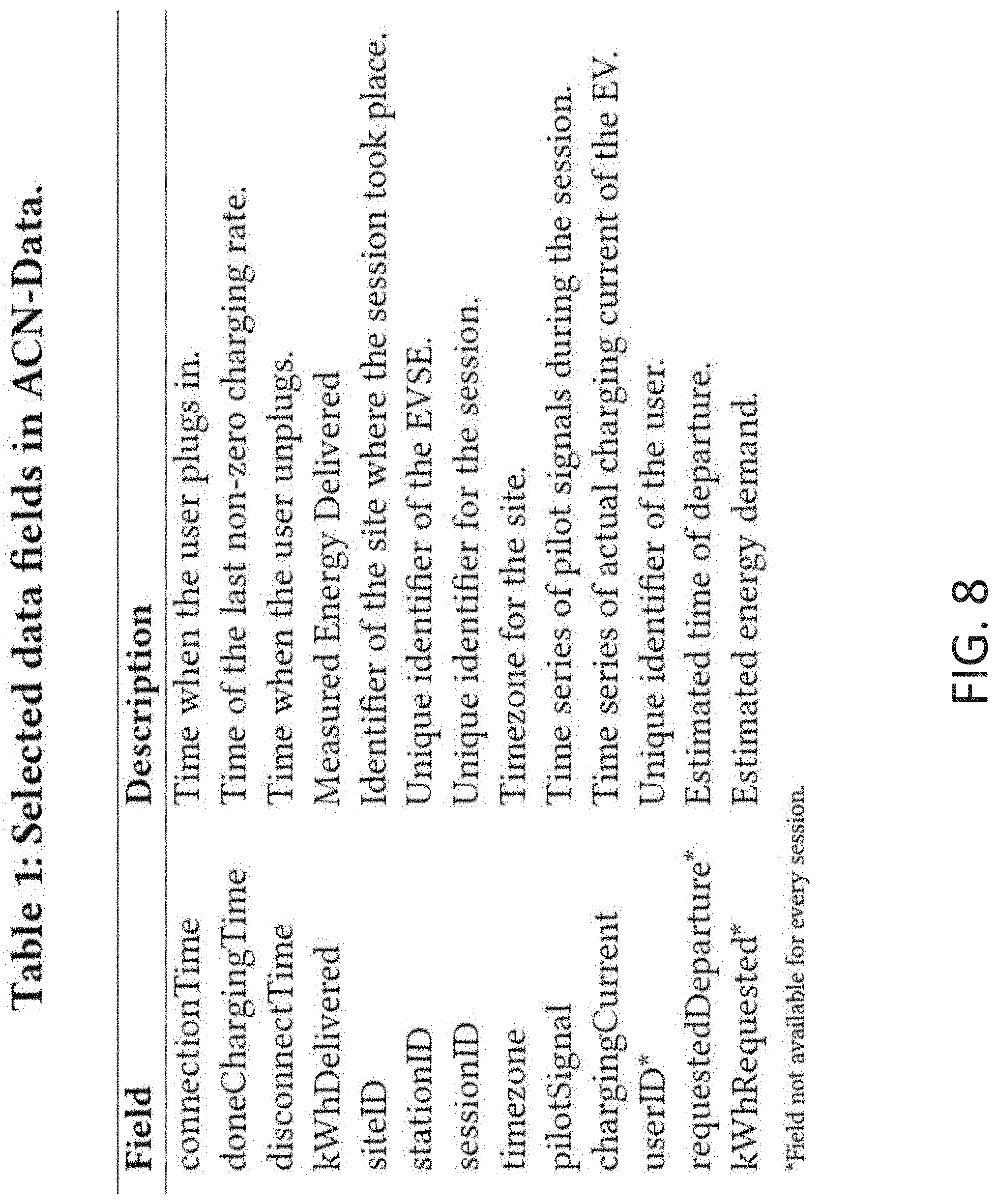
[0030] FIG. 8 shows a table which describes some of relevant data collected in accordance with an embodiment, of the invention.
[0031] FIG. 9 shows data collected for a number of sessions from multiple sites in accordance with an embodiment of the invention.
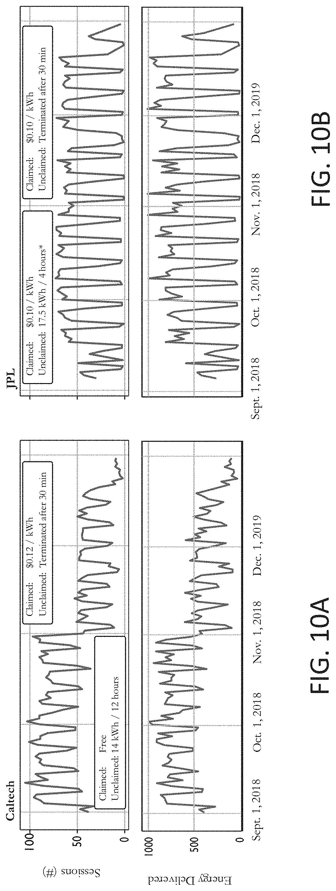
[0032] FIG. 10A shows system utilization data for the California Institute of Technology (Caltech) site in accordance with an embodiment of the invention. FIG. 10B shows system utilization data for NASA's Jet Propulsion Laboratory (JPL) site in accordance with an embodiment of the invention.
[0033] FIG. 11A shows distributions of weekday arrivals and departures for Caltech in accordance with an embodiment of the invention. The graph on the left is data for free charging and the graph on the right is data for paid charging. FIG. 11B shows distributions of weekend arrivals and departures for Caltech in accordance with an embodiment of the invention. The graph on the left is data for free charging and the graph on the right is data for paid charging. FIG. 11C shows distributions of weekday arrivals and departures for JPL in accordance with an embodiment of the invention.
[0034] FIG. 12A shows a weekday distribution of initial laxities for Caltech site in accordance with an embodiment of the invention. FIG. 12B shows a weekend distribution of initial laxities for Caltech in accordance with an embodiment of the invention. FIG. 12C shows a weekday distribution of initial laxities for JPL site in accordance with an embodiment of the invention.
[0035] FIG. 13A shows a comparison of uncontrolled capacity and optimally scheduled capacity required for Caltech in accordance with an embodiment of the invention. FIG. 13B shows a comparison of uncontrolled capacity and optimally scheduled capacity required for JPL in accordance with an embodiment of the invention.
[0036] FIG. 14A shows a comparison of modelled arrivals and departure distributions with actual data for Caltech during a training period in accordance with an embodiment of the invention. FIG. 14B shows a comparison of modelled energy, delivered with actual data for Caltech during a training period in accordance with an embodiment of the invention.
[0037] FIG. 15A shows individual and population Gaussian mixture models (GMM) prediction errors for Caltech duration as a function of look tack period in accordance with an embodiment of the invention. FIG. 15B shows individual and population GMM prediction errors for Caltech energy as a function of look back period in accordance with an embodiment of the invention. FIG. 15C shows individual and population GMM prediction errors for JPL duration as a function of look back period in accordance with an embodiment of the invention. FIG. 151) shows individual and population GMM prediction errors for JPL energy as a function of look back period in accordance with an embodiment of the invention.
[0038] FIG. 16 shows average symmetric mean absolute percentage error (SMAPE) for a JPL data set in accordance with an embodiment of the invention.
[0039] FIG. 17 shows a table which displays the average SMAPEs for various methods tested in accordance with an embodiment, of the invention.
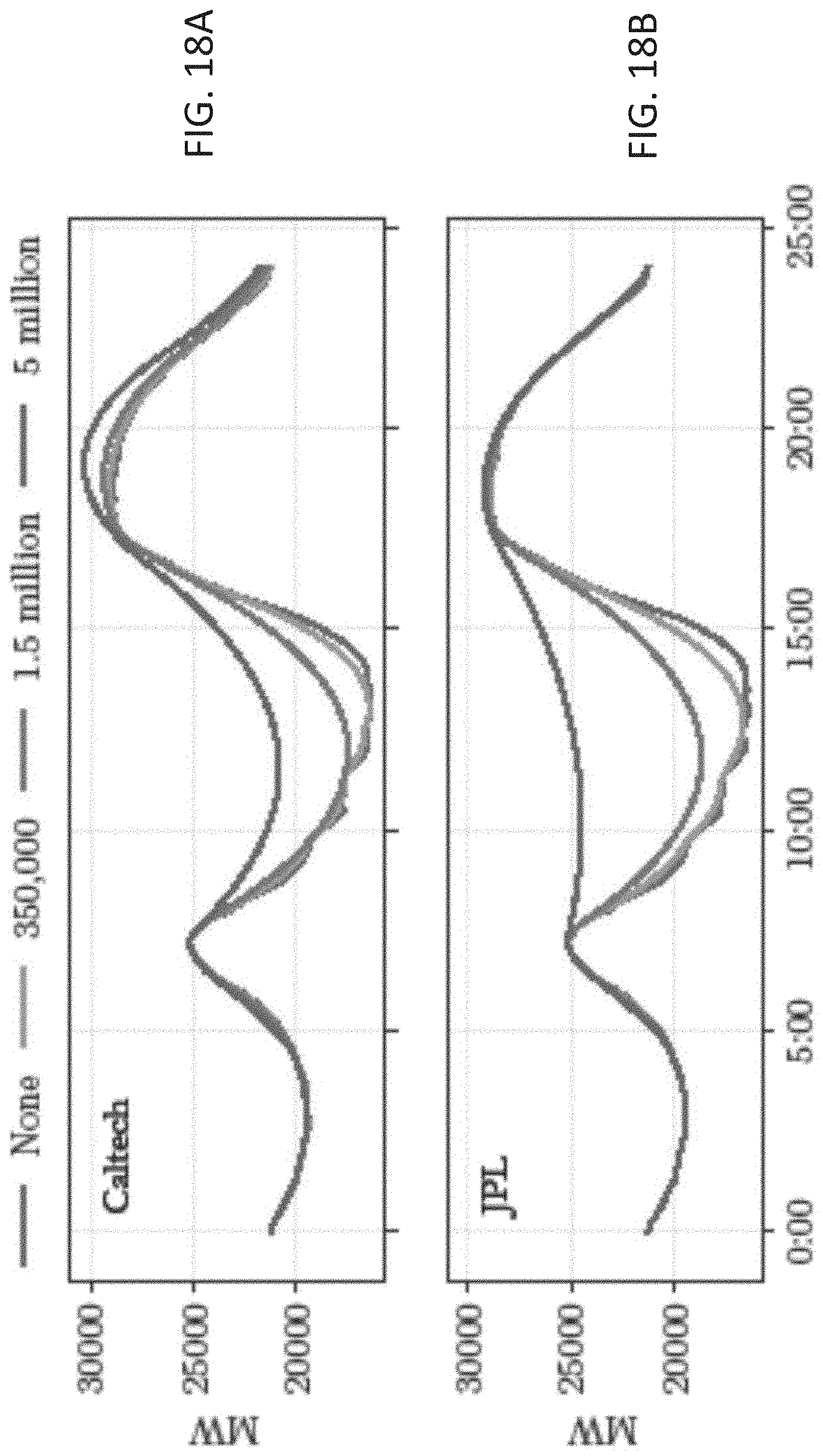
[0040] FIG. 18A shows net energy demand curves after optimal smoothing for Caltech in accordance with an embodiment of the invention. FIG. 18B shows net energy demand curves after optimal smoothing for JPL in accordance with an embodiment of the invention.
[0041] FIG. 19A shows up ramp rate as a function of number of EVs in accordance with an embodiment of the invention. FIG. 19B shows down ramp rate as a function of number of EVs in accordance with an embodiment of the invention. FIG. 19C shows peak demand as a function of number of EVs in accordance with an embodiment of the invention.
DETAILED DESCRIPTION
[0042] Turning now to the drawings, systems and methods for adaptive EV charging in accordance with embodiments of the invention are illustrated. In many embodiments, systems and methods for adaptive EV charging can use adaptive charging network (ACN) data collected from EV charging physical infrastructure sites located in various localities in order to simulate EV charging control routines, and then push out updated EV charging control routines to one or more of EV charging physical infrastructure sites. In several embodiments, systems and methods for adaptive EV charging can be utilized to collect data from electric vehicle supply equipment (EVSEs) or charging stations, aggregate the collected data in a cloud based system, analyze the collected data to arrive at new charging processes, and then push out the new charging processes to the EV chargers. In many embodiments, systems and methods for adaptive EV charging can be used to gather EV charging data, to utilize the underlying distribution of charging session parameters in order to train models of EV user behaviors, and control the charging of a vehicle based upon those models in smart and reliable processes that are not relied upon EV user's inputs. In several embodiments, systems and methods for adaptive EV charging can be used for controlling charging of large numbers of electric vehicles in order to alleviate steep ramping conditions caused by the so called Duck curve, and utilize user data to smooth EV energy demand over the course of a day, and therefor smooth out the Duck curve. In many embodiments, systems and methods for adaptive EV charging can include a processor, and a memory containing: an adaptive EV charging application; a plurality of EV charging parameters, where the processor is configured to learn an underlying model of an electric vehicle's battery charging behavior. EV power distribution networks and methods of controlling the charging of EVs in accordance with various embodiments of the invention are discussed further below.
Electric Vehicle Power Distribution Networks
[0043] A power distribution network in accordance with an embodiment of the invention is shown in FIG. 1. Electricity is generated at power generator 102. Power transmission lines 104 can transmit electricity between the power generator and power substation 106. Power substation 106 additionally can connect to one or more large storage batteries 108, which temporarily store electricity, as well as power distribution lines 110. The power distribution lines 110 can transmit electricity from the power substation to one or more charging stations 112. Charging station 112 can include a battery 114, and/or solar panels 116. Electric vehicles 118 can connect to the charging station and request charging.
[0044] The power generator 102 can represent a power source including (but not limited to) those using fossil fuels, nuclear, solar, wind, or hydroelectric power. Substation 106 changes the voltage of the electricity for more 19 efficient power distribution. Solar panels 116 are distributed power generation sources, and can generate power to supply electric charging stations as well as generate additional power for the power grid.
[0045] While specific systems incorporating a power distribution network are described above with reference to FIG. 1, any of a variety of systems including adaptive EV charging can be utilized to provide adaptive EV charging as appropriate to the requirements of specific applications in accordance with various embodiments of the invention. Cloud based adaptive EV charging application in accordance with a number of embodiments of the invention are discussed below.
Cloud Based Adaptive EV Charging Application
[0046] A cloud based adaptive EV charging application in accordance with an embodiment of the invention is shown in FIG. 2. In several embodiments, one or more electric vehicles can connect to electric vehicle supply equipment (EVSE) 212 and request charging. In the illustrated embodiment, systems and methods for adaptive EV charging include at least a processor 202, an I/O interface 204 and memory 206. In many embodiments, the memory can include software including adaptive EV charging application 208 as well as charging parameters 210. In many embodiments, the adaptive EV charging application 208 can collect data from the EVSE regarding EV charging patterns. The adaptive EV charging application 208 can provide a charging control routine to the EVSE in accordance with an embodiment of the invention. The adaptive EV charging application 208 can calculate charging parameters by using a combination of its own EV parameters, and/or adaptive EV charging parameters.
[0047] While specific systems incorporating cloud based adaptive EV charging application are described above with reference to FIG. 2, any of a variety of systems can be utilized to provide a cloud based adaptive EV charging application as appropriate to the requirements of specific applications in accordance with various embodiments of the invention. Adaptive EV charging platforms that include ACN data collection, ACN simulation and/or control routine push-out in accordance with a number of embodiments of the invention are discussed further below.
ACN Data Collection, ACN Simulation and Control Routine Push-Out
[0048] An adaptive EV charging platform including ACN data collection, ACN simulation and control routine push-out in accordance with an embodiment of the invention is shown in FIG. 3. In several embodiments, the adaptive EV charging platform can collect ACN data from one or more EVSEs, simulate control routines, and then push out updated control processes to one or more ETVSEs. In many embodiments, the adaptive EV charging platform can receive user parameters in order to update the control routines. A flow chart illustrating a process for gathering EV user data, simulating control routines, and pushing out updated EV charging control routines in accordance with an embodiment of the invention is shown in FIG. 4. An overview of the process for adaptive EV charging is illustrated in FIG. 4. EV user data is gathered 402 and fed to 404, where control routines are simulated. Updated control routines are pushed-out to EVSEs 406.
[0049] While specific systems incorporating an adaptive EV charging platform including ACN data collection, ACN simulation and control routine push-out are described above with reference to FIGS. 3 and 4, any of a variety of systems can be utilized to provide an adaptive EV charging platform including ACN data collection, ACN simulation and control routine push-out as appropriate to the requirements of specific applications in accordance with various embodiments of the invention. A process for receiving EV user request and delivering optimum charge in accordance with a number of embodiments of the invention are discussed further below.
Process for Receiving EV User Request and Delivering Optimum Charge
[0050] A flow chart illustrating a process for receiving an EV user request for charging and delivering optimum charge to the EV user in accordance with an embodiment of the invention is shown in FIG. 5. In many embodiments, an adaptive EV charging process can receive a request for charging from an EV user 502. An amount of energy and a duration for delivering that energy to the EV user is determined using the adaptive EV charging process 504. The time-varying charging rate based on time of day and electric system load is determined 506. The adaptive EV charging process then synchronizes with an EVSE to deliver optimum charge to the EV user 508.
[0051] While specific systems incorporating a flow chart illustrating a process for receiving an EV user request for charging and delivering optimum charge are described above with reference to FIG. 5, any of a variety of systems can be utilized incorporating a flow chart illustrating a process for receiving an EV user request for charging and delivering optimum charge for the requirements of specific applications in accordance with various embodiments of the invention. Usage of EV driver laxity to oversubscribe EVSEs in accordance with a number of embodiments of the invention are discussed further below.
Use of EV Driver Laxity to Oversubscribe EVSEs
[0052] EV driver laxity can be used to oversubscribe charging infrastructure, such as, but not limited to, transformers, cables, and utility interconnections, in accordance with an embodiment of the invention as shown in FIGS. 6A and 6B. In certain embodiments, a conventional charging process can exceed a power limit of an EVSE during peak charging hours as illustrated in FIG. 6A. Adaptive EV charging can control charging of EVs such that a power limit of EVSE is not exceeded in accordance with an embodiment of the invention as illustrated in FIG. 6B.
[0053] While specific systems incorporating use of EV driver laxity to oversubscribe EVSEs are described above with reference to FIGS. 6A and 6B, any of a variety of systems can be utilized to provide use of EV driver laxity to oversubscribe EVSEs for the requirements of specific applications in accordance with various embodiments of the invention. Demand met by adaptive charging compared to other charging methods in accordance with a number of embodiments of the invention are discussed further below.
Comparison of Adaptive EV Charging to Other Methods
[0054] Adaptive charging can increase the amount of demand met compared to other charging methods in accordance with an embodiment of the invention as illustrated in FIG. 7. In accordance with an embodiment of the invention, demand met by adaptive charging exceeds all other methods of charging as a function of transformer capacity.
[0055] While specific systems comparing demand met by adaptive charging to other charging Methods are described above with reference to FIG. 7, any of a variety of systems can be utilized to provide a comparison of demand met by adaptive charging to other charging methods for the requirements of specific applications in accordance with various embodiments of the invention. Adaptive charging network data examples in accordance with a number of embodiments of the invention are discussed further below.
Adaptive Charging Network Data Examples
[0056] ACN data was collected from two adaptive charging networks located in California in accordance with an embodiment of the invention. The first location was Caltech campus and the second location was the Jet Propulsion Laboratory (JPL). The Caltech site includes a parking garage and has 54 EVSEs along with a 50 kW de fast charger. The Caltech site is open to the public and is often used by non-Caltech EV drivers. Since the parking garage is near the campus gym, many drivers charge their EVs while working out in the morning or evening. JPL's site includes 52 EVSEs in a parking garage. In contrast to the Caltech site, access to the JPL site is restricted and only employees are able to use the charging system. The JPL site is representative of workplace charging while the Caltech site is a hybrid between workplace and public use charging. EV penetration is also quite high at JPL. `I`his leads to high utilization of the EVSEs as s well as an impromptu program where drivers move their EVs after they have finished charging to free up plugs for other drivers. In both cases, to reduce capital costs, infrastructure elements such as transformers have been oversubscribed. Note that the specific number of EVSEs can vary.
[0057] In many embodiments, an adaptive scheduling routine is used to deliver each driver's requested energy prior to her stated departure time without exceeding the infrastructure capacity. An offline version of the adaptive charging routine that assumes full knowledge of all EV arrival times, departure times, and energy demands in advance in accordance with a number of embodiments of the invention is discussed further below.
Offline Adaptive Charging Routine
[0058] In certain embodiments, let V be the set of all EVs over all optimization horizon :={1 . . . T}. Each EV i.di-elect cons.V can be described, by a tuple (a.sub.i, e.sub.i, d.sub.i, r.sub.i) where a.sub.i is the EV's arrival time relative to the start of the optimization horizon, e.sub.i is its energy demand, d.sub.i is the duration of the session, and r.sub.i is the maximum charging rate for EV i. The charging rates for each EV in each period solve the following problem:
SCH ( , U , ) : min r ^ U ( r ^ ) s . t . r ^ .di-elect cons. ##EQU00001##
where the optimization variable r:=(r.sub.i(1), . . . , r.sub.i(T), i.di-elect cons.V) defines the scheduled charging rates of each EV over the optimization horizon . The utility function U(r) encodes the operator's objectives and the feasible set the various constraints.
[0059] To illustrate, the objective
U ( r ) := i .di-elect cons. T i .di-elect cons. ( t - T ) r i ( t ) ##EQU00002##
is used to encourage EVs to finish charging as quickly as possible, freeing up capacity for future arrivals. In several embodiments, a feasible set takes the form
0 .ltoreq. r i ( t ) .ltoreq. r _ i a i .ltoreq. t < a i + d i , i .di-elect cons. ( 1 a ) r i ( t ) = 0 t < a i , t .gtoreq. a i + d i , i .di-elect cons. ( 1 b ) t = a i d i - 1 r i ( t ) .ltoreq. e i i .di-elect cons. ( 1 c ) f j ( r 1 ( t ) , , r N ( t ) ) .ltoreq. I l ( t ) t .di-elect cons. , l .di-elect cons. ( 1 d ) ##EQU00003##
[0060] Constraints (1a) ensure that charging rate are non-negative and below their maximum r.sub.i(1); (1b) ensure that an EV does not charge before its arrival or after its departure time; (1c) limits the total energy delivered to EV i to at most e.sub.i; and (1d) enforce a set of given infrastructure limits I.sub.l(t) indexed by l.di-elect cons..
[0061] In many embodiments, if the utility function is strictly decreasing in all elements of r, if it is feasible to meet all EV's energy demands, then constraint (1c) is observed to be tight. In general, it is possible that the energy delivered may not reach the user's requested energy due to their battery becoming full or congestion in the system.
ACN Data Collected
[0062] In many embodiments, ACN platform can enable the collection of detailed data about each charging session which occurs in the system. FIG. 8 shows a table which describes some of the relevant, data collected in accordance with an embodiment of the invention. In several embodiments, in order to obtain data directly from users, a mobile application can be utilized. In certain embodiments, a driver can first scan a quick response (QR) code on the EVSE which allows the adaptive EV charging application to associate the driver with a particular charging session. The driver can then input her estimated departure time and requested energy. This can be referred to as user input data. In certain embodiments, when a user does not use the mobile application, default values for energy requested and duration can be assumed and no user identifier may be attached to the session. In several embodiments, sessions with an associated user input can be referred to as claimed and those without as unclaimed.
[0063] In several embodiments, adaptive EV charging can focus on a 3-tuple (a.sub.i, d.sub.i, e.sub.i) in collected data for both user input and an actual measured behavior. Number of sessions collected from each site per month as well as whether these sessions were tagged with a user's input, i.e. claimed, is shown in FIG. 9 in accordance with an embodiment of the invention. Claimed sessions are useful for studying individual user behavior.
Understanding User Behavior
System Utilization
[0064] EVSE utilization, specifically number of sessions served and amount of energy delivered each day, together with pricing information, and default parameters for unclaimed sessions are shown in FIG. 10A (Caltech) and FIG. 10B (JPL) in accordance with an embodiment of the invention. FIGS. 10A and 10B show that both sites display a cyclic usage pattern with much higher utilization during weekdays than on weekends, as expected for workplace charging. Furthermore, Caltech site, being a university and an open campus, has non-trivial usage on weekends. In contrast, JPL, as a closed campus, has next to no charging on weekends and holidays.
[0065] The data confirms the difference between paid and free charging facilities. During the first 2.5 years of operation the Caltech site EV charging was free for drivers. However, beginning Nov. 1, 2018, a fee of $0.12/kWh was imposed. This date can clearly be seen in FIG. 10A, as both the number of sessions per day and daily energy delivered decreased significantly. Because of an issue with site configuration, approximately half of the EVSEs at JPL, were free prior to Nov. 1, 2018. However at the JPL site, large decrease in utilization in terms of number of sessions or energy delivered after November 1 is not observed. This is likely due to the fact that demand for charging is high enough to overshadow any price sensitivity.
Arrival and Departure Data
[0066] Distributions of arrivals and departures for Caltech on weekdays and weekends for free charging and paid charging, and JPL on weekdays are shown in FIGS. 11A, 11B and 11C in accordance with an embodiment of the invention. For Caltech, the shape of the distributions are similar before and after paid charging was implemented. Two key differences can be noted in weekday charging between free and paid periods. First, the second peak around 6 pm vanishes. This is attributed to a decrease in community usage of the Caltech site after its charging costs became comparable to at-home charging. Second, the peak in arrivals (departures) around 8 am (5 pm) increases. This is expected as instituting paid charging has reduced community usage in the evening which leads to a higher proportion of users displaying standard work schedules.
[0067] The weekday arrival distribution has a morning peak at both sites. For conventional charging system, these peaks necessitate a larger infrastructure capacity and lead to higher demand charges. In addition, as EV adoption grows, the se morning spikes in demand could prove challenging for utilities as well. As expected, departures are analogous to arrivals. They begin to increase as the workday ends, with peaks in the period 5-6 pm at both Caltech and JPL. Departures at JPL tend to begin earlier, which is consistent with the earlier arrival times while departures at Caltech tend to stretch into the night owing to the heterogeneity of individual schedules as well as later arrivals. Since the Caltech site is open to the public and is located on a university campus, it is used on the weekends as well. Arrivals and departures are much more uniform on weekends for both the unpaid and paid periods. This uniformity is due to the aggregation of many highly heterogeneous weekend schedules.
Driver and System Flexibility
Driver Laxity
[0068] The initial laxity of an EV charging session i is defined as
LAX ( i ) = d i - i r _ i ##EQU00004##
LAX(i)=0 means that EV i must be charged at its maximum rate r, over the entire duration d.sub.i of its session in order to meet its energy demand e.sub.i. A higher value of LAX(i) means there is more flexibility in satisfying its energy demand.
[0069] Distribution of initial laxities are shown in FIGS. 12A (Caltech weekday), 12B (Caltech weekend) and 12C (JPL weekday) in accordance with an embodiment of the invention. For weekdays most EVs display high laxity. On weekends laxity tends to be lower as EV users tend to want to get charged and get on with their day. One way to quantify the aggregate flexibility of a group of EVs is the minimum system capacity needed to meet all their charging demands. A smaller system capacity requires a lower capital investment and operating cost for a charging operator. To calculate the minimum system capacity, SCH(V, U.sub.cap, ) is solved for optimal charging rates r*, for each day in the data-set where V is the set of all EVs using the charging system in a day,
U cap ( r ) := max t i .di-elect cons. r i ( t ) ##EQU00005##
and is equivalent to (1) except that (1c) is strengthened to equality. For simplicity, any infrastructure constraints (1d) in is not considered. The distribution of the minimum system capacity U.sub.cap(r*) per day in the data set is shown in FIGS. 13A (Caltech) and 13B (JPL). It shows that the adaptive EV charging platform would have been able to meet the demand for 100% of days in the data et with just 60 kW of capacity for Caltech and 84 kW for JPL, while conventional uncontrolled systems of the same capacity would only be able to meet demand on 22% and 38% of days respectively. For reference Caltech has an actual system capacity of 150 kW and JPL has 195 kW.
Learning User Behavior
[0070] In many embodiments, an underlying joint distribution of characteristics including (but not limited to) arrival time, session duration, and energy delivered based upon Gaussian mixture models (GMMs) is utilized. In several embodiments, the GM Ms are used to predict user behavior, optimally size onsite solar for adaptive EV charging, and control EV charging to smooth the so called Duck curve.
[0071] In certain embodiments, adaptive EV charging can utilize a GMM as a second-order approximation to the underlying distribution. An ACN data set can be modeled as follows to fit a GMM. Consider a data set X consisting of N charging sessions. The data for each session i=1, . . . , is represented by a triple x.sub.i=(a.sub.i, d.sub.i, e.sub.i) in R.sup.3 where a.sub.i denotes the arrival time, d.sub.i denotes the duration and e.sub.i is the total energy (in kWh) delivered. The data point X; are independently and identically distributed (i.i.d.) according to some unknown distribution. In practice, each driver in a workplace environment exhibits only a few regular patterns. For example, on weekdays, a driver may typically arrive at 8 am and leave around 6 pm, though her actual arrival and departure times may be randomly perturbed around their typical values. On weekends, driver behavior may change such that the same driver may come around noon. Therefore, let K be the number of typical profiles denoted by .mu..sub.1, . . . , .mu..sub.K. Each data point X.sub.i can be regarded a corrupted version of a typical profile with a certain probability. Define a latent variable Y.sub.i.ident.k if and only if X.sub.i is corrupted from .mu..sub.k. Moreover, by the i.i.d. assumption, each incoming EV has an identical probability .PHI..sub.k taking .mu..sub.k, i.e., .PHI..sub.k:=(Y.sub.i=k) for i=1, . . . N, k=1, . . . , K. Conditioned on Y.sub.i=k, the difference X.sub.i-.mu..sub.k that the profile X.sub.i deviates from the typical profile .mu..sub.k can be regarded as Gaussian noise. In this manner, assuming Y.sub.i=k.sub.i let X.sub.i.about.(.mu..sub.k, .SIGMA..sub.k) be a Gaussian random variable with mean .mu..sub.k and covariance matrix .SIGMA..sub.k. To estimate the underlying distribution and approximate it as a mixture of Gaussian distributions, it suffices to estimate the parameters .theta.=(.PHI..sub.k, .mu..sub.k, .SIGMA..sub.k).sub.K=1.sup.K. The probability density of observing a data point x can then be approximated using the learned GMM as
p ( x .theta. ) = k = 1 K .phi. k exp ( - x - .mu. k k - 1 2 / 2 ) ( 2 .phi. ) 3 det ( k ) ##EQU00006##
Population and Individual-Level GMMs
[0072] In many embodiments, adaptive EV charging can train GMMs based on a training data set X.sub.Train, and predict the charging duration and energy delivered for drivers in a set .mu.. The results are tested on a corresponding testing data set X.sub.Test. As illustrated in FIG. 9, the training data collected at both Caltech and JPL can be divided into two parts: user-claimed data X.sub.C and unclaimed data X.sub.U.
[0073] In certain embodiments, two different approaches are considered. A first, approach generates a population-level GMM (P-GMM) based on the overall training data X.sub.Train=X.sub.C.orgate.X.sub.U. However, users can have distinctive charging behaviors. To achieve better prediction accuracy, adaptive EV charging can take advantage of the user-claimed data and predict the charging duration and energy delivered for each individual user. In a second approach, the claimed data can be partitioned into a collection of smaller data sets consisting of the charging information of each user in .mu.. Therefore, X.sub.C=.orgate..sub.j.di-elect cons..mu.X.sub.j. Adaptive EV charging can then train individual-level GMMs (1-GMM) for each user j.di-elect cons..mu. by fine tuning the weights of the components of the P-GM M with data from each of the users to arrive at a final model for each of them.
Distribution Learned by P-GMM
[0074] In certain embodiments, to evaluate the accuracy of adaptive EV charging's learned population-level GMM with respect to an underlying distribution, 100,000 samples were gathered from a P-GMM trained on data from Caltech site prior to Sep. 1, 2018. The data is plotted in FIG. 14A (distribution of these samples) and in FIG. 14B (empirical distribution from the training set). Departure time was plotted instead of duration directly as it demonstrates that adaptive EV charging model has learned not only the distribution of session duration but also the correlation between arrival time and duration. It can be seen in all cases that adaptive EV charging learned distribution matches the empirical distribution well.
Predicting User Behavior
[0075] In several embodiments, adaptive EV charging can utilize a GMM that has been learned from the ACN data set to predict a user's departure time and the associated energy consumption based on that user's known arrival time. Adaptive EV charging data shows that user input can be quite unreliable, partially because of a lack of incentives for users to provide accurate predictions. In many embodiments, adaptive EV charging platform shows that the predictions can be more precise using simple probabilistic models.
Calculating Arrival Time-Based Predictions
[0076] Let denote the set of users. Suppose a convergent solution .theta..sup.(j)=(.PHI..sub.k.sup.(j), .mu..sub.k.sup.(j), .SIGMA..sub.k.sup.(j)).sub.k=1.sup.K is obtained for user j.di-elect cons. where .mu..sub.k.sup.(j):=(a.sub.k.sup.(j), k.sub.k.sup.(j), e.sub.k.sup.(j)) and the user's arrival time is known a priori as .sup.(j). For the sake of completeness, the following formulas are used for predicting a duration d.sup.(j) and energy to be delivered .sup.(j) as conditional Gaussians of the user j.di-elect cons..mu.:
d _ ( j ) = k = 1 K .phi. k - ( j ) ( d k ( j ) + ( a ~ ( j ) - a k ( j ) ) k ( j ) ( 1 , 2 ) k ( j ) ( 1 , 1 ) ) ( 2 ) e _ ( j ) = k = 1 K .phi. k - ( j ) ( e k ( j ) + ( a ~ ( j ) - a k ( j ) ) k ( j ) ( 1 , 3 ) k ( j ) ( 1 , 1 ) ) ( 3 ) ##EQU00007##
where .SIGMA..sub.k.sup.(j)(1, 1), .SIGMA..sub.k.sup.(j)(1, 2) and .SIGMA..sub.k.sup.(j)(1, 3) are the first, second and third entries in the first column (or row) of the co-variance matrix .SIGMA..sub.k.sup.(j) respectively. Denoting by p(|.mu., .sigma..sup.2) the probability density for a normal distribution with mean .mu. and variance .sigma..sup.2, the modified weights conditioned on arrival time in (2) and (3) above are
.phi. _ k := p ( a ~ ( j ) a k ( j ) , k ( j ) ( 1 , 1 ) ) k = 1 K p ( a ~ ( j ) a k ( j ) , k ( j ) ( 1 , 1 ) ) ##EQU00008##
Error Metrics
[0077] In many embodiments, both absolute error and percentage error are considered when evaluating duration and energy predictions.
[0078] Recall that is the set of all users in a testing data set X.sub.Test. Let .sub.j denote the set of charging sessions for user j.di-elect cons.. The Mean Absolute Error (MAE) is defined in (4) to assess the overall deviation of the duration and energy consumption. For a testing data set X.sub.Test={(a.sub.i,j, d.sub.i,j, e.sub.i,j)}.sub.j.di-elect cons..mu.,i.di-elect cons..sub.j, the corresponding MAEs for duration and energy are represented by MAE(d) and MAE(e) with
MAE ( x ) := j .di-elect cons. 1 i .di-elect cons. j 1 j x i , j - x ^ i , j ( 4 ) ##EQU00009##
where {circumflex over (x)}.sub.i,j is the estimate of x.sub.i,j and x=d or c.
[0079] In several embodiments, a symmetric mean absolute percentage error (SMAPE) can be used to avoid skewing the overall error by the data points wherein the duration and energy consumption take small values. The corresponding SMAPEs for duration and energy are represented by SMAPE(d) and SMAPE(e) with
SMAPE ( x ) := j .di-elect cons. 1 i .di-elect cons. j 1 j x i , j - x ^ i , j x i , j + x ^ i , j .times. 100 % ( 5 ) ##EQU00010##
Results and Discussion
[0080] In accordance with an embodiment of the invention, MAE(d) and MAE(e) for I-GMM and P-GMM on Caltech data set are illustrated in FIGS. 15A, 15B, 15C and 15D as a function of the look back period which defines the length of the training set. Users with larger than 20 sessions during Nov. 1, 2018 and Jan. 1, 2019 are included in and tested. Note that the size of the training data may not be proportional to the length of periods since in general there is less claimed session data early in the data set as shown in FIGS. 10A, 10B, and 10C. The 30-day testing data was collected from Dec. 1, 2018 to Jan. 1, 2019. Performance of prediction accuracy with different training data size was analyzed by training the GMMs with data collected from five time intervals ending on Nov. 30, 2018 and starting on Sep. 1, 2018, Sep. 15, 2018, Oct. 1, 2018, Oct. 15, 2018 and Nov. 1, 2018 respectively. The GMM components are initialized using k-means clustering as implemented by the Scikit learn GMM package. Since it is not deterministic, this initialization can be repeated a number of times (e.g. 25 times) and the model with the highest log-likelihood on the training data set selected. Grid search and cross validation can be used to find the best number of components for each GMM. As can readily be appreciated, the specific process utilized for initializing the GMM is largely dependent upon the requirements of a specific application.
[0081] As illustrated in FIGS. 15A, 15B, 15C and 15D, for the JPL data set with testing data obtained from Dec. 1, 2018 to Jan. 1, 2019, the 60-day training data gives the best overall performance. This is in agreement with user behavior changing over time and there is a trade-off between data quality and size. The Caltech data set also displays this trade-off; however, the best performance was found for only a 30-day training set. This is likely because there was a transition from free to paid charging on November 1, which meant that data prior to that date had very different properties.
[0082] Hence, for the JPL data set, adaptive EV charging can fix the training data as the one collected from Oct. 1, 2018 to Dec. 1, 2018 and show the scatterings of SMAPEs for each session in the testing data (from Dec. 1, 2018 to Jan. 1, 2019) in FIG. 16. The SMAPEs are concentrated on small values with a few outliers and high-quality duration prediction has a positive correlation with high-quality energy prediction. As a comparison, user input SMAPEs, shown as Xs, are much worse.
[0083] FIG. 17 shows a table which displays the average SMAPEs for the various methods tested in accordance with an embodiment of the invention. For Caltech and JPL, the results displayed use the 30 and 60-day training data respectively. For reference the error is also calculated for two additional ways to predict user parameters: 1) a mean of the training data X.sub.j is used as adaptive EV charging prediction for each user, 2) user input data is utilized directly as the prediction. Note that to account for stochasticity in the GMM training process, the results in FIGS. 15A, 15B, 15C, and 15D and FIG. 17 are obtained via 50 Monte Carlo simulations.
[0084] User input data conspicuously gives the least accurate overall prediction. In certain embodiments, significant improvements are me made by leveraging tools from statistics and machine learning to better predict user behaviors, e.g., using GMMs.
Solar Sizing
[0085] In many embodiments, collection of ACN data and training of models can be utilized to determine the sizing of solar arrays in the manner described in the U.S. Provisional Patent Application Ser. No. 62/803,157 entitled "Date-Driven Approach To Joint EV And Solar Optimization Using Predictions" to Zachary J. Lee et. al., filed Feb. 8, 2019, and in the U.S. Provisional Patent Application Ser. No. 62/964,504 entitled "EV Charging Optimization Using Adaptive Charging Network Data" to Zachary J. Lee et. al., filed Jan. 22, 2020, the disclosures of which are herein incorporated by reference in their entirety.
Smoothing the Duck Curve
[0086] In several embodiments, adaptive EV charging platform can utilize user data to smooth the EV energy demand over the course of the day and therefore smooth out the Duck curve. In certain embodiments, adaptive EV charging platform can be used for controlling the charging of large number of EVs in order to alleviate the steep ramping conditions caused by the Duck curve.
[0087] In certain embodiments, the problem of minimizing ramping can be formulated as
SCH(V,U.sub.ramp,) (6)
where the objective is denoted by
U ramp := t .di-elect cons. ( D ^ ( t ) - D ^ ( t - 1 ) ) 2 ( 7 ) and D ^ ( t ) := i .di-elect cons. r i ( t ) + D ( t ) ( 8 ) ##EQU00011##
[0088] Here D(t) is the net demand placed on the grid after non-dispatchable renewable energy is subtracted from the total demand. In certain embodiments, flexible loads such as water heaters, appliances, pool pumps, etc. are treated as being fixed.
Case Studies
[0089] In many embodiments, adaptive EV charging platform can be utilized to analyze a net demand curve from California independent system operator (CAISO). For example, for the 2018 case analysis, three levels of EV penetration in California were analyzed based on the current number of EVs in California (350,000) and the state's goals for 2025 (1.5 million) and 2030 (5 million). For this case analysis, an optimistic assumption can be made that all of the electric vehicles would be available for workplace charging. The length of each discrete time interval is set in the optimization to be 15 min.
[0090] In several embodiments, to reduce the computational burden in solving (6) for millions of EVs, a representative sample of n EVs can be used drawn from the learned distribution and scale down the net demand curve D(t) from CAISO by the ratio of a to the desired number of EVs, denoted by N. Define {circumflex over (D)}(t):=(n/N){tilde over (D)}(t). (6)-(8) can be solved for D(t) and this representative sample. Finally, the optimal net demand curve can be scaled, {circumflex over (D)}*(t), by N/n to arrive at a final curve in the original units. For this experiment, n=1,000.
[0091] FIGS. 18A and 18B show the resulting optimal net demand curves {circumflex over (D)}*(t), for both the Caltech data and the JPL data. Even with only 350,000 EVs, a non-trivial smoothing can be observed of the net demand curve. With 1.5 million EVs under control, a significant filling of the "belly" of the duck can be observed as well as a reduction in the morning and afternoon ramping requirements. By the time 5 million EVs under control is reached, an almost complete smoothing of the duck can be observed in the JPL case. Note that for the Caltech distribution, 5 million EVs lead to a noticeable increase in peak demand. This is due to fact that the distribution used for free charging includes a significant number of short sessions that begin around 5-7 pm, thus requiring adaptive EV charging platform to charge the EVs during the peak of background demand. This demonstrates benefits of concentrat-ing EV charging during normal working hours, for which the JPL distribution is representative.
Quantitative Results
[0092] In many embodiments, in order to determine the amount of smoothing of the Duck curve, the number of EVs under control can be varied from 10,000 to 10 million for each distribution. Each group EVs can be scheduled by using (6) and measuring the resulting maximum up and down ramps as well as the peak demand. The results are shown in FIGS. 19A, 19B, and 19C.
[0093] In several embodiments, with as few as 2 million EVs under control, up and down ramping can be reduced by nearly 50% with only a 0.6% increase in peak demand when using the JPL distribution.
Data-Based Battery Fitting
[0094] In many embodiments, a model for an EV battery can be fitted using charging data for a given EV. In several embodiments, using a transformation of charging time series into the energy domain, data processing techniques, and model fitting techniques, a piecewise function can be fitted to a battery that captures different modes of battery charging behavior.
Battery Model in Energy Domain
[0095] In many embodiments, ACN data can provide useful information on charging sessions, including time series for pilot: (charging) signal and charging rate, and energies requested and delivered. In certain embodiments, battery models can be fitted depending on objectives. In several embodiments, a best fit battery model is employed using a time series data. In many embodiments, a piecewise linear 2-stage model can be fitted for a battery. Fitting to this battery model entails finding optimal values for the parameters r.sup.max and h, where r.sup.max is the maximum charging rate in the constant charging regime and h is the threshold state of charge at which decrease in charging rate begins. In certain embodiments, the problem can be analyzed in the energy domain, in which case the governing equation becomes:
r _ ( e ^ ) = { r max e ^ + e ( 0 ) .ltoreq. e h r max ( e _ - e ^ - e ( 0 ) e _ - e h ) e ^ + e ( 0 ) > e h ##EQU00012##
[0096] For a given session, , e.sup.h, e(0), and Y are energy delivered, threshold energy, initial energy, and battery capacity respectively.
[0097] Looking at one session and assuming initial energy is 0, rewriting the governing equation as
r _ ( e ^ ) = { r max e ^ .ltoreq. e h r max + ( - r max e _ - e h ) e ^ - ( - r max e _ - e h ) e h e ^ > e h ##EQU00013##
3 parameters can be fitted in a linear regression on a piecewise linear equation: e.sup.h, r.sup.max, and a slope that depends on (and the other parameters).
Generating Energy Domain Data
[0098] In many embodiments, ACN data provides a time series of charging rate and pilot signal. For the purposes of this fitting, charging rates for which the pilot signal was not binding can be used; that is, the pilot signal was some threshold above the charging rate. For these charging rates, the battery is charging at its maximum possible rate at that time, and charging rates can be used in the battery fitting. For charging rates within some threshold of the pilot signal, it is unknown if the charging rate is limited by the pilot signal, thus those rates cannot be used to determine a maximal charging rate profile. Further, EVs may spend a significant amount of time charging at 0A while having a nonzero pilot signal (due to the deadband at 6A or the pilot setpoint at 8A). Thus, charging rates of 0A are also not considered.
[0099] In several embodiments, once a time series of nonzero charging rates is obtained which is not bound by the pilot signal, these charging rates can be converted into an energy delivered vs. charging rat graph. Each charging rate can have a time over which it was applied, which, when combined with the charger voltage, provides a time series of energy delivered. This can then be plotted against charging rate.
[0100] In many embodiments, despite the aforementioned time series processing, noisy behavior is still present in the charging profile. Much of this behavior consists of sudden dips in the charging signal (i.e. over just one timestep). Because the battery equation is piecewise linear, median filtering will preserve the functional form of the charging profile (in the energy domain), while also being robust to window size. In certain embodiments, a median filter is used, but other filtering methods may also be used to bring the data closer to the appropriate functional form. For example, the charging rate in the energy domain is not expected to ever increase significantly (after accounting for the pilot signal), therefore a filter based on that criterion may also be utilized.
Fitting Over Multiple Sessions
[0101] In many embodiments, after obtaining a clean charging rate vs. energy delivered curve, an optimization library can be used such as scipy.optimize to fit the energy domain battery equation to the data, yielding parameter values for e.sup.h, r.sup.max, and . If this is the only session for this user, the analysis can be stopped at this point with a battery model associated with only this session. However, with multiple sessions per user an even more accurate battery model can be obtained. Note that in the single-session fitting, battery initial charge of 0 is assumed.
[0102] In many embodiments, for multiple sessions for a single user, assuming that the single user has one vehicle (and thus one battery), each individual session can be fitted for the user, and then the energy domain charging profile for each session can be shifted such that the e.sup.h's are aligned to the maximum e.sup.h over all sessions. For instance, if one session yielded an e.sup.h of 1 kWh, while another yielded 4 kWh, all the points of the first session would be shifted by 3 kWh. This is akin to assigning an initial charge to the battery for each session, with one session (the session that sets the max e.sup.h) having an initial charge of 0 kWh. After this shifting is done for all sessions for a given user, the fit to the model is done again, this time with data from all sessions.
[0103] In certain embodiments, the resultant fit gives accurate parameters for the battery's governing equations for one user under some model assumptions. In many embodiments, fitted parameters for a session (along with an initial energy estimate yielded by the shifting step) may be associated with that session in ACN data, and this fitted data may then be used in simulation, such that accurate charging based on real user charging behavior is obtained. The models for these batteries may be included in a model predictive control or other optimization framework to improve scheduling. In several embodiments, the fidelity of these fitted models may be tested by feeding the recorded pilot signals from ACN data into a ACN-Sim simulator (or another simulator). Also, as this process yields battery parameters for each user, clusters of users with similar batteries can be determined, and those clusters can be used to improve simulation models, match users to car models, or assign batteries to unclaimed, unfittable sessions following a distribution learned from the battery parameter clusters. At the individual user level, battery models could be used to infer metrics such as battery health.
Possible Relaxations
[0104] In many embodiments, a user having multiple charging sessions is not necessary if one trace demonstrates most battery modes of behavior. Even if this isn't the case, an accurate model can be found that captures some of the battery behavior (like max charging rate), which is better than blind guessing. In several embodiments, this process can be employed for battery models other than linear 2 stage. Fitting to different functions may require different data processing and curve matching techniques. In certain embodiments, the data pre-processing (accounting for the pilot signal, median filtering, etc.) is only one possible pipeline for this analysis. Different filters, fitting directly to the time series, removing different parts of the charging rate data, etc. are all possible alternatives. In certain embodiments, an actual fitting process uses linear regression to find optimal parameters. Likewise, the shifting step, in which the threshold energy parameters for each session are aligned, may be done by matching other parameters, such as x intercept or max rate, or by fitting each session to an aggregate session curve calculated from all sessions, recording the optimal shifts used to match each session to the aggregate curve. The general idea in that step is to somehow align the data from all sessions to yield an aggregate data set for which fitting to a single set of parameter values makes sense.
Worst-Case Linear Two Stage Battery Fitting
[0105] In certain embodiments, such as when data is noisy, sparse, or unclaimed, or in certain simulations focusing on tail behavior, charging sessions are mapped to a worst-case scenario in which tail-behavior is maximized. Then the battery fitting objectives are twofold. First, given an energy delivered and a duration of the stay, the minimum total battery capacity is to be calculated such that it is feasible to deliver the requested energy within the specified duration when charging at maximum rate. Second, given that the minimum feasible total battery capacity was calculated, the maximum initial charge is determined such that a requested energy is delivered for this battery. In many embodiments, an amount of time the battery charges is increased in the non-ideal region, allowing an easier analysis of the effects of battery tail behavior on EV charging.
[0106] In several embodiments, assuming that charging is always at the maximum possible rate, the maximum rate of charge can be express r (in amps) as the rate equation
r _ ( .zeta. ) = { r max .zeta. .ltoreq. h r max ( 1 - .zeta. 1 - h ) .zeta. > h ##EQU00014##
Here, r.sup.max is the maximum rate of charge under ideal conditions, (is the state of charge of the battery, and h is the battery state of charge at which the battery transitions from ideal to non-ideal behavior, also known as the threshold or transition state of charge. If the maximum battery capacity is given and the voltage of charging V in volts, the above equation can be expressed in terms of the rate of change of state of charge. To do this, note that
.zeta. . max = .differential. .zeta. .differential. t = r max V 1000 e _ ##EQU00015##
assuming is in kWh. Then, the rate equation may be rewritten in terms of the rate of change of state of charge .zeta.:
.zeta. . _ = { .zeta. . max .zeta. .ltoreq. h .zeta. . max ( 1 - .zeta. 1 - h ) .zeta. > h ##EQU00016##
[0107] This is a differential equation with two cases that depend on the initial condition .zeta.(0)=.zeta..sub.0. In the first case, if .zeta..sub.0>h, the only governing differential equation that applies is
.zeta. . _ = .zeta. . max ( 1 - .zeta. 1 - h ) ##EQU00017## .zeta. ( 0 ) = .zeta. 0 ##EQU00017.2##
which has the solution
.zeta. ( t ) = 1 + exp ( .zeta. . max t h - 1 ) ( .zeta. 0 - 1 ) ##EQU00018##
[0108] In the second case, .zeta..sub.0.ltoreq.h and there are two individual differential equations to solve with different initial conditions. First, solve .zeta.=.zeta..sub.max with initial condition .zeta.(0)=.zeta..sub.0, which has solution .zeta.(t)=.zeta..sup.maxt+.zeta..sub.0. Thus,
.zeta. . _ = .zeta. . max ( 1 - .zeta. 1 - h ) ##EQU00019## .zeta. ( h - .zeta. 0 .zeta. . max ) = h ##EQU00019.2##
[0109] The reason for the above initial condition is that the second differential equation starts taking effect when .zeta..gtoreq.h. The ideal region was charged up until this point, the time at which this transition occurs is (h-.zeta..sub.0)/.zeta..sup.max and at this time .zeta.(t)=h. This differential equation has solution
.zeta. ( t ) = 1 + exp ( .zeta. . max t + .zeta. 0 - h h - 1 ) ( h - 1 ) ##EQU00020##
[0110] Combining all the equations, the following formula is arrived at for state of charge as a function of initial charge .zeta..sub.0 and charging time t assuming charging is performed at the maximum possible .zeta.:
.zeta. ( .zeta. 0 , t ) = { .zeta. . max t + .zeta. 0 .zeta. 0 < h , t .ltoreq. h - .zeta. 0 .zeta. . max 1 + exp ( .zeta. . max t + .zeta. 0 - h h - 1 ) ( h - 1 ) .zeta. 0 < h , t > h - .zeta. 0 .zeta. . max 1 + exp ( .zeta. . max t h - 1 ) ( .zeta. 0 - 1 ) .zeta. 0 .gtoreq. h ##EQU00021##
[0111] The problem discussed at the beginning of this section can be restated as, given a fixed .DELTA..zeta. and t (and assuming the other constants are fixed), find the maximum (o such that .zeta.(.zeta..sub.0, t)-.zeta..sub.0.gtoreq..DELTA..zeta.. Although there is a way to solve this problem in a closed form, it is simpler and more stable to solve this problem in steps, outlined below:
1. Assume .zeta..sub.0.gtoreq.h. Then,
.zeta. ( .zeta. 0 , t ) = 1 + exp ( .zeta. . max t h - 1 ) ( .zeta. 0 - 1 ) ##EQU00022## .zeta. ( .zeta. 0 , t ) - .zeta. 0 = ( exp ( .zeta. . max t h - 1 ) - 1 ) ( .zeta. 0 - 1 ) = .DELTA. .zeta. ##EQU00022.2## [0112] Note that in this case, .DELTA.s.sub.t(.zeta..sub.0) (that is, .zeta.(.zeta..sub.0, t)-.zeta..sub.0 with constant t) is decreasing in .zeta..sub.0, as the coefficient of .zeta..sub.0 is negative (h-1<0). Thus, finding the minimum .zeta..sub.0 is equivalent to finding the .zeta..sub.0 for which exactly .DELTA..zeta. state of charge is delivered. Inverting the above expression for .DELTA.s.sub.t(.zeta..sub.0), thus
[0112] .zeta. 0 = ( exp ( .zeta. . max t h - 1 ) - 1 ) - 1 ##EQU00023## [0113] .zeta..sub.0 can be calculated directly, and then checked if the assumption that .zeta..sub.0.gtoreq.h holds. If so, the answer has been found. If not, it is known that .zeta..sub.0<h and must consider the other two cases of the expression for .zeta.. 2. Assuming .zeta..sub.0<h and writing the piecewise conditions in terms of .zeta..sub.0, thus:
[0113] .DELTA. s t ( .zeta. 0 ) = { .zeta. . max t .zeta. 0 .ltoreq. h - .zeta. . max t 1 + exp ( .zeta. . max t + .zeta. 0 - h h - 1 ) ( h - 1 ) - .zeta. 0 .zeta. 0 > h - .zeta. . max t ##EQU00024##
[0114] In certain embodiments, the maximal .zeta..sub.0.gtoreq.h-.zeta..sup.maxt in known because if .zeta..sub.0 were any lower, the same amount of energy would be delivered, since .zeta..sup.maxt does not depend on .zeta..sub.0. Thus
.DELTA. s t ( .zeta. 0 ) = 1 + exp ( .zeta. . max t + .zeta. 0 - h h - 1 ) ( h - 1 ) - .zeta. 0 ##EQU00025##
[0115] This function can be inverted if special functions are used (namely, the product log, or Lambert W function) but such functions are unstable in the range of possible inputs, so instead, a search for an optimal .zeta..sub.0 is done. First, note the following:
.differential. .DELTA. .zeta. .differential. .zeta. 0 = exp ( .zeta. . max t + .zeta. 0 - h h - 1 ) - 1 .ltoreq. 0 ##EQU00026##
[0116] Since .zeta..sub.0.gtoreq.h-.zeta..sup.maxt, .zeta..sup.maxt+.zeta..sub.0-h.gtoreq.0 and .delta..DELTA..zeta./.delta..zeta..sub.0 is always negative (except the edge of the search interval, .zeta..sub.0=h-.zeta..sup.maxt, where it is 0). Since .DELTA.s.sub.t(.zeta..sub.0) is decreasing in .zeta..sub.0, find the .zeta..sub.0 such that .DELTA.s.sub.t(.zeta..sub.0)=.DELTA..zeta.. In certain embodiments, this can be done by binary search since the function searched for is decreasing. Thus, a maximum .zeta..sub.0 is obtained efficiently.
Linear 2 Stage Battery Charging
[0117] Given an initial state of charge (j, a charging duration t (t=1 if a charge for one period is performed), a threshold h, a capacity , a voltage V, and a maximum charging rate r.sup.max, the battery state of charge is determined after t periods as:
.zeta. ( .zeta. 0 , t ) = { .zeta. . max t + .zeta. 0 .zeta. 0 < h , t .ltoreq. h - .zeta. 0 .zeta. . max 1 + exp ( .zeta. . max t + .zeta. 0 - h h - 1 ) ( h - 1 ) .zeta. 0 < h , t > h - .zeta. 0 .zeta. . max 1 + exp ( .zeta. . max t h - 1 ) ( .zeta. 0 - 1 ) .zeta. 0 .gtoreq. h .zeta. . max = r max V 1000 e _ ##EQU00027##
[0118] Although the present invention has been described in certain specific aspects, many additional modifications and variations would be apparent to those skilled in the art. It is therefore to be understood that the present invention can be practiced otherwise than specifically described including systems and methods for adaptive EV charging without departing from the scope and spirit of the present invention. Thus, embodiments of the present invention should be considered in all respects as illustrative and not restrictive. Accordingly, the scope of the invention should be determined not by the embodiments illustrated, but by the appended claims and their equivalents.
* * * * *
D00000
D00001
D00002
D00003
D00004
D00005
D00006
D00007
D00008
D00009
D00010
D00011
D00012

D00013

D00014

D00015

D00016

D00017

D00018
D00019


P00001

P00002

P00003

P00004

P00005

P00006

P00007

P00008

XML
uspto.report is an independent third-party trademark research tool that is not affiliated, endorsed, or sponsored by the United States Patent and Trademark Office (USPTO) or any other governmental organization. The information provided by uspto.report is based on publicly available data at the time of writing and is intended for informational purposes only.
While we strive to provide accurate and up-to-date information, we do not guarantee the accuracy, completeness, reliability, or suitability of the information displayed on this site. The use of this site is at your own risk. Any reliance you place on such information is therefore strictly at your own risk.
All official trademark data, including owner information, should be verified by visiting the official USPTO website at www.uspto.gov. This site is not intended to replace professional legal advice and should not be used as a substitute for consulting with a legal professional who is knowledgeable about trademark law.