Systems, Apparatus, Methods, And Architecture For Precision Heterogeneity In Accelerating Neural Networks For Inference And Trai
Sharma; Hardik ; et al.
U.S. patent application number 16/744037 was filed with the patent office on 2020-07-16 for systems, apparatus, methods, and architecture for precision heterogeneity in accelerating neural networks for inference and trai. This patent application is currently assigned to Bigstream Solutions, Inc.. The applicant listed for this patent is Bigstream Solutions, Inc.. Invention is credited to Jongse Park, Hardik Sharma.
| Application Number | 20200226444 16/744037 |
| Document ID | 20200226444 / US20200226444 |
| Family ID | 71516690 |
| Filed Date | 2020-07-16 |
| Patent Application | download [pdf] |


View All Diagrams
| United States Patent Application | 20200226444 |
| Kind Code | A1 |
| Sharma; Hardik ; et al. | July 16, 2020 |
SYSTEMS, APPARATUS, METHODS, AND ARCHITECTURE FOR PRECISION HETEROGENEITY IN ACCELERATING NEURAL NETWORKS FOR INFERENCE AND TRAINING
Abstract
For one embodiment, a hardware accelerator with a heterogenous architecture for training quantized neural networks is described. In one example, a hardware accelerator for training quantized data, comprises memory to store data, a plurality of compute units to perform computations of a data type for an inference phase of training quantized data of a neural network, and plurality of heterogenous precision compute units to perform computations of mixed precision data types for a backward propagation phase of training quantized data of the neural network.
| Inventors: | Sharma; Hardik; (Mountain View, CA) ; Park; Jongse; (Mountain View, CA) | ||||||||||
| Applicant: |
|
||||||||||
|---|---|---|---|---|---|---|---|---|---|---|---|
| Assignee: | Bigstream Solutions, Inc. Mountain View CA |
||||||||||
| Family ID: | 71516690 | ||||||||||
| Appl. No.: | 16/744037 | ||||||||||
| Filed: | January 15, 2020 |
Related U.S. Patent Documents
| Application Number | Filing Date | Patent Number | ||
|---|---|---|---|---|
| 62792785 | Jan 15, 2019 | |||
| Current U.S. Class: | 1/1 |
| Current CPC Class: | G06F 5/06 20130101; G06N 3/084 20130101; G06F 9/5027 20130101; G06N 20/00 20190101; G06N 5/046 20130101; G06F 9/4881 20130101; G06N 3/10 20130101; G06N 3/04 20130101; G06F 9/5061 20130101; G06N 3/08 20130101 |
| International Class: | G06N 3/04 20060101 G06N003/04; G06N 3/08 20060101 G06N003/08; G06N 3/10 20060101 G06N003/10 |
Claims
1. A hardware accelerator for training quantized data, comprising: memory including multilevel memory hierarchy to store data; and a plurality of heterogenous precision compute units coupled to the memory, the plurality of heterogenous precision compute units to perform computations of mixed precision data types for training and inference in neural networks (NN).
2. The hardware accelerator of claim 1, further comprising: a first systolic array having a first type of heterogeneous precision compute units; a second systolic array having a second type of heterogeneous precision compute units; and a third systolic array having a third type of heterogeneous precision compute units.
3. The hardware accelerator of claim 3, wherein the first type of heterogeneous precision compute units support 32 bit floating point precision, the second type of heterogeneous precision compute units support 16 bit fixed point precision, and the third type of heterogeneous precision compute units support binary precision.
4. The hardware accelerator of claim 1, wherein the plurality of heterogenous precision compute units comprise mixed-precision bit width multiply-accumulate computation units that support a flexible range of precision for floating point and fixed point inputs including activations in a forward phase of training quantized data and gradients in the backward propagation phase.
5. The hardware accelerator of claim 1, further comprising: a fourth systolic array having the plurality of heterogenous precision compute units including a first type of precision compute units, a second type of precision compute units, and a third type of precision compute units.
6. The hardware accelerator of claim 1, wherein the plurality of heterogenous precision compute units perform computations on mixed precision datatypes without converting a low bit width precision datatype into a high bit width precision datatype to improve performance and energy-efficiency.
7. The hardware accelerator of claim 1, wherein the plurality of heterogenous precision compute units dynamically match varying precision requirements of NN training.
8. A data processing system comprising: a hardware processor; and a hardware accelerator that includes a plurality of heterogenous symmetric precision compute units and asymmetric precision compute units to perform computations of mixed precision data types for a backward propagation phase of training quantized data of a neural network.
9. The data processing system of claim 8, wherein the hardware accelerator is implemented on a Field Programmable Gate Array (FPGA).
10. The data processing system of claim 8, wherein the heterogenous symmetric precision compute units include a first compute unit to support a first type of precision for first and second operands and a second compute unit to support a second type of precision for third and fourth operands.
11. The data processing system of claim 9, wherein the heterogenous asymmetric precision compute units include a first compute unit to support a first type of precision for a first and operand and a second type of precision for a second operand.
12. The data processing system of claim 8, wherein the heterogenous asymmetric precision compute units include a second compute unit to support a third type of precision for a first and operand and a fourth type of precision for a second operand.
13. The data processing system of claim 8, wherein the plurality of heterogenous asymmetric precision compute units comprise mixed-precision bit width multiply-accumulate computation units that support a flexible range of precision for floating point and fixed point inputs including activations in a forward phase of training quantized data and gradients in the backward propagation phase.
14. The data processing system of claim 8, wherein the plurality of heterogenous asymmetric precision compute units perform computations on mixed precision datatypes without converting a low bit width precision datatype into a high bit width precision datatype to improve performance and energy-efficiency.
15. The data processing system of claim 8, further comprising: a first systolic array having heterogenous asymmetric precision compute units that support a first type of precision for a first operand and a second type of precision for a second operand; and a second systolic array having heterogenous asymmetric precision compute units that support a third type of precision for a first operand and a fourth type of precision for a second operand.
16. A hardware accelerator for training quantized data, comprising: memory including multilevel hierarchy to store data; and a plurality of heterogenous precision compute units coupled to the memory, the plurality of heterogenous precision compute units to perform computations of mixed precision data types for a backward propagation phase of training quantized data of the neural network (NN); and software-programmable precision, wherein the precision for the plurality of heterogenous precision compute units to vary dynamically and be programmed through software.
17. The hardware accelerator of claim 16, wherein the computations are performed on the mixed precision datatypes without converting a low bit width precision datatype into a high bit width precision datatype.
Description
RELATED APPLICATIONS
[0001] This application claims the benefit of U.S. Provisional Application No. 62/792,785, filed on Jan. 15, 2019, the entire contents of this Provisional application is hereby incorporated by reference.
TECHNICAL FIELD
[0002] Embodiments described herein generally relate to the fields of data processing and machine learning, and more particularly relates to a hardware accelerator having a heterogenous architecture for training quantized neural networks.
BACKGROUND
[0003] While interest in Deep Neural Networks (DNNs) continues to grow for big data applications, the focus of recent literature has shifted towards exploring efficient ways of training and executing deep learning models. One prominent approach for improving efficiency is quantization, which reduces the bit widths for data and operations in a deep learning model to yield increased performance and/or energy efficiency. From the architecture community, several prior approaches have exploited quantization to improve the efficiency of the inference phase of deep learning. In order to maximize the benefits from quantization and retain classification accuracy, the quantized version of the DNNs needs to be retrained which can take weeks on GPUs, depending on the size of the DNN model.
SUMMARY
[0004] For one embodiment of the present invention, a hardware accelerator with a heterogenous architecture for training quantized neural networks is described. In one example, a hardware accelerator for training quantized data, comprises memory to store data, a plurality of compute units to perform computations of a data type for an inference phase of training quantized data of a deep neural network, and plurality of heterogenous precision compute units to perform computations of mixed precision data types for a backward propagation phase of training quantized data of the neural network.
[0005] Other features and advantages of embodiments of the present invention will be apparent from the accompanying drawings and from the detailed description that follows below.
BRIEF DESCRIPTION OF THE DRAWINGS
[0006] FIG. 1 shows an embodiment of a block diagram of a big data system 100 for providing big data applications for a plurality of devices in accordance with one embodiment.
[0007] FIGS. 2A and 2B illustrate methods for training quantized DNNs with a hardware accelerator architecture (e.g., homogenous architecture in FIG. 2A, heterogenous architecture in FIG. 2B) in accordance with one embodiment.
[0008] FIG. 3A illustrates pooling layers for the inference phase in accordance with one embodiment.
[0009] FIG. 3B illustrates pooling layers 370 for the back-propagation phase in accordance with one embodiment.
[0010] FIG. 4 illustrates an architecture 400 that includes three distinct types of computational blocks 410, 420, and 430 that are specialized for the different types of operations for training quantized DNNs in accordance with one embodiment.
[0011] FIG. 5 illustrates a homogeneous accelerator architecture 500 in accordance with one embodiment.
[0012] FIG. 6 illustrates the design of a compute unit in accordance with one embodiment.
[0013] FIG. 7 illustrates adder logic 700 that utilizes a novel low-overhead desynchronized encoding for zero-skipping in accordance with one embodiment.
[0014] FIG. 8 illustrates non-zero detection logic 800 that includes zero-detector logic 810 and non-zero selector 820 in accordance with embodiment.
[0015] FIG. 9 illustrates scheduling operations across multiple MPZS-arrays in accordance with one embodiment.
[0016] FIG. 10 illustrates an overview of a DNN workflow 1000 in accordance with one embodiment.
[0017] FIGS. 11 and 12 illustrate performance of the GPU platform in comparison to different variations of the present design as implemented in a FPGA platform in accordance with one embodiment.
[0018] FIG. 13 illustrates the schematic diagram of a data processing system according to an embodiment of the present invention.
[0019] FIG. 14 illustrates the schematic diagram of a multi-layer accelerator according to an embodiment of the invention.
[0020] FIG. 15 is a diagram of a computer system including a data processing system according to an embodiment of the invention.
[0021] FIG. 16 shows the details of the specialized circuit 1700 for accelerating neural networks in prior art.
[0022] FIG. 17 shows the details of the CU 1800 in the systolic array circuit in accordance with one embodiment.
[0023] FIG. 18 summarizes the taxonomy 1900 of the different strategies for heterogeneous precision in the circuit for computations in Neural Network training and inference.
[0024] FIG. 19 shows the first method, called coarse-grained heterogeneous precision 1911 in accordance with one embodiment.
[0025] FIG. 20 shows the second method, called fine-grained heterogeneous precision 1912 in accordance with another embodiment.
[0026] In one implementation of symmetric heterogeneous precision 1903 circuit, FIG. 21 shows an example of a systolic array 2200 that can operate on two multidimensional arrays of data, with either both multidimensional arrays of data being floating-point 2201 or both multidimensional arrays of data are binary precision 2205.
[0027] In one implementation of asymmetric heterogeneous precision 1902 circuit, FIG. 22 shows examples of a systolic array 2300 that can operate on two multidimensional arrays of data, with the precision of both multidimensional arrays of data being different.
[0028] FIG. 23 shows one embodiment of software-configurable flexible precision 1907, which is a circuit 2400 that can match the precision requirements for the multidimensional arrays of data in Neural Network dynamically to execute the various training and inference operations in Neural Networks.
[0029] Built upon our reference design, described in circuits 2000, 2100, 2200, 2300, and 240o, this specification provides exemplary acceleration designs by taking a design choice per each dimension of precision heterogeneity as one embodiment of this specification in FIG. 24.
[0030] FIG. 25 shows the details of the CU 2511, implemented in the asymmetric software-programmable circuit 2510.
[0031] FIG. 26 shows the data and operations for quantized Neural Network training for a single convolution layer in accordance with one embodiment.
DETAILED DESCRIPTION OF EMBODIMENTS
[0032] Methods and systems having a heterogenous architecture for training quantized neural networks are described. The present design leverages two algorithmic properties: quantization and sparsity for quantized training. Training operations for quantized DNNs possess dual characteristics: (1) due to high sparsity in the high precision gradients, the backward phase favors sparse execution, and (2) the quantized activations/weights in the forward phase favor dense execution due to the large overhead of zero-skipping for quantized activations. The present design provides a unified architecture that leverages both properties and shows that FPGAs not only provide higher energy efficiency than GPUs, and FPGAs can, on average, outperform GPUs across a range of quantization techniques and DNN topologies.
[0033] In the following description, for purposes of explanation, numerous specific details are set forth in order to provide a thorough understanding of the present invention. It will be apparent, however, to one skilled in the art that the present invention can be practiced without these specific details. In other instances, well-known structures and devices are shown in block diagram form in order to avoid obscuring the present invention.
[0034] Reference in the specification to "one embodiment" or "an embodiment" means that a particular feature, structure or characteristic described in connection with the embodiment is included in at least one embodiment of the present invention. Thus, the appearances of the phrase "in one embodiment" appearing in various places throughout the specification are not necessarily all referring to the same embodiment. Likewise, the appearances of the phrase "in another embodiment," or "in an alternate embodiment" appearing in various places throughout the specification are not all necessarily all referring to the same embodiment.
[0035] The following glossary of terminology and acronyms serves to assist the reader by providing a simplified quick-reference definition. A person of ordinary skill in the art may understand the terms as used herein according to general usage and definitions that appear in widely available standards and reference books.
[0036] HW: Hardware.
[0037] SW: Software.
[0038] I/O: Input/Output.
[0039] DMA: Direct Memory Access.
[0040] CPU: Central Processing Unit.
[0041] FPGA: Field Programmable Gate Arrays.
[0042] CGRA: Coarse-Grain Reconfigurable Accelerators.
[0043] GPGPU: General-Purpose Graphical Processing Units.
[0044] MLWC: Many Light-weight Cores.
[0045] ASIC: Application Specific Integrated Circuit.
[0046] PCIe: Peripheral Component Interconnect express.
[0047] CDFG: Control and Data-Flow Graph.
[0048] FIFO: First In, First Out
[0049] NIC: Network Interface Card
[0050] HLS: High-Level Synthesis
[0051] Dataflow analysis: An analysis performed by a compiler on the CDFG of the program to determine dependencies between a write operation on a variable and the consequent operations which might be dependent on the written operation.
[0052] Accelerator: a specialized HW/SW component that is customized to run an application or a class of applications efficiently.
[0053] In-line accelerator: An accelerator for I/O-intensive applications that can send and receive data without CPU involvement. If an in-line accelerator cannot finish the processing of an input data, it passes the data to the CPU for further processing.
[0054] Bailout: The process of transitioning the computation associated with an input from an in-line accelerator to a general purpose instruction-based processor (i.e. general purpose core).
[0055] Continuation: A kind of bailout that causes the CPU to continue the execution of an input data on an accelerator right after the bailout point.
[0056] Rollback: A kind of bailout that causes the CPU to restart the execution of an input data on an accelerator from the beginning or some other known location with related recovery data like a checkpoint.
[0057] Gorilla++: A programming model and language with both dataflow and shared-memory constructs as well as a toolset that generates HW/SW from a Gorilla++description.
[0058] GDF: Gorilla dataflow (the execution model of Gorilla++).
[0059] GDF node: A building block of a GDF design that receives an input, may apply a computation kernel on the input, and generates corresponding outputs. A GDF design includes of multiple GDF nodes. A GDF node may be realized as a hardware module or a software thread or a hybrid component. Multiple nodes may be realized on the same virtualized hardware module or on a same virtualized software thread.
[0060] Engine: A special kind of component such as GDF that contains computation.
[0061] Infrastructure component: Memory, synchronization, and communication components.
[0062] Computation kernel: The computation that is applied to all input data elements in an engine.
[0063] Data state: A set of memory elements that contains the current state of computation in a Gorilla program.
[0064] Control State: A pointer to the current state in a state machine, stage in a pipeline, or instruction in a program associated to an engine.
[0065] Dataflow token: Components input/output data elements.
[0066] Kernel operation: An atomic unit of computation in a kernel. There might not be a one to one mapping between kernel operations and the corresponding realizations as states in a state machine, stages in a pipeline, or instructions running on a general purpose instruction-based processor.
[0067] Two challenges for accelerating training for quantized DNNs have been identified including high precision for gradients and variation in computations. Gradients in the backward phase of training include both the backward propagation of loss and the calculation of weight gradients, compared to activations and weights for forward propagation. From a hardware perspective, the higher precision requirements for gradients means that an accelerator for training quantized DNNs would limit the benefits from quantizing the DNNs.
[0068] In regards to variation in computations, the highly parallel multiply add operations for convolutions/fully-connected layers are interleaved with quantization transformations and require expensive transcendental functions such as tan h or sigmoid that operate on floating-point data.
[0069] While it can be argued that the transcendental functions and the data movement operations can be offloaded to the host CPU, the latency for data-transfer for every convolution in the DNN can limit the benefits from acceleration. Furthermore, the quantization transformation and even the data-representations (e.g., fixed-point, power-of-2, floating-point) vary significantly across the different techniques proposed in recent literature, making ASIC acceleration approach less appealing. To overcome the challenges mentioned above, the present design targets FPGAs for their flexibility and develops a heterogenous architecture, which is an accelerator for training quantized DNNs. This heterogenous architecture is designed to challenge the reign of GPUs as the de facto platform for DNN training. The heterogenous architecture leverages three algorithmic properties of quantized DNN training algorithms.
[0070] In one example, compute intensive operations for the convolution and fully-connected layers in quantized training need mixed precision; that is, one of the operands is a high-precision gradient while the other is a quantized weight/activation. Using mixed-precision allows the heterogenous architecture to reduce the high resource cost of the compute units, increasing the parallelism that the FPGA can offer using its limited pool of resources.
[0071] In another example, training operations for quantized DNNs possess a dual characteristic--the high-precision gradients in the backward phase are highly sparse (>99% zeros); while the quantized activations in the forward phase have between 45-60% zeroes. The heterogenous architecture leverages the dual characteristics of high-precision, high-sparsity in the backward phase and low-precision, low-sparsity in the forward phase.
[0072] In another example, both the data-representations (fixed-point, power of 2, etc.) and precision (number of bits) for activations, weights, and gradients vary between different DNN models. The heterogenous architecture utilizes a template architecture that exploits the reconfigurability of the FPGA to generate a specialized implementation for each quantized DNN.
[0073] The heterogenous architecture acting as an accelerator utilizes the properties of quantization in the bit-heterogeneous architecture to deliver significant improvement in performance and energy efficiency over GPUs. The quantization transformation and the quantized data representation both differ for different training algorithms. However, the structure of the compute intensive convolution/activation layers remain the same. To support a wide range of quantization transformations, and yet, provide high performance for a wide range of DNNs, the heterogenous architecture uses (1) systolic arrays (e.g., sparse dense heterogenous architecture array) for the highly parallel mixed-precision Multiply-Accumulate (MAC) operations in convolution/fully-connected layers in a DNN, and (2) programmable data Transformation Arrays (TX-array) to support the resource intensive quantization transformations as well as the activation/pooling layers in DNNs.
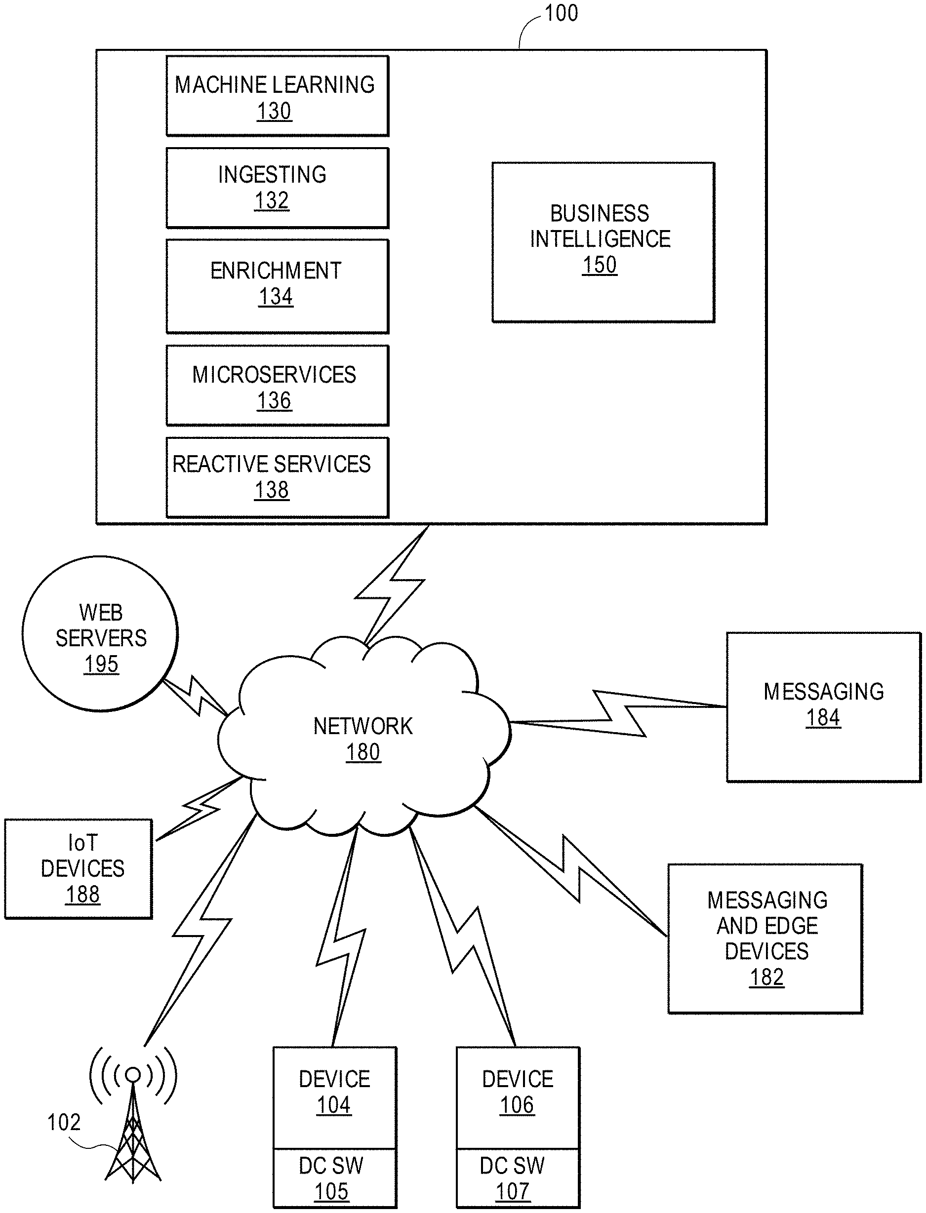
[0074] FIG. 1 shows an embodiment of a block diagram of a machine learning system 100 for providing machine learning applications for a plurality of devices in accordance with one embodiment. The machine learning system 100 includes machine learning modules 130 (e.g., DNN modules), ingestion layer 132, enrichment layer 134, microservices 136 (e.g., microservice architecture), reactive services 138, and business intelligence layer 150. In one example, a microservice architecture is a method of developing software applications as a suite of independently deployable, small, modular services. Each service has a unique process and communicates through a lightweight mechanism. The system 100 provides big data services by collecting data from messaging systems 182 and edge devices, messaging systems 184, web servers 195, communication modules 102, internet of things (IoT) devices 186, and devices 104 and 106 (e.g., source device, client device, mobile phone, tablet device, laptop, computer, connected or hybrid television (TV), IPTV, Internet TV, Web TV, smart TV, satellite device, satellite TV, automobile, airplane, etc.). Each device may include a respective big data application 105, 107 (e.g., a data collecting software layer) for collecting any type of data that is associated with the device (e.g., user data, device type, network connection, display orientation, volume setting, language preference, location, web browsing data, transaction type, purchase data, etc.). The system 100, messaging systems and edge devices 182, messaging systems 184, web servers 195, communication modules 102, internet of things (IoT) devices 186, and devices 104 and 106 communicate via a network 180 (e.g., Internet, wide area network, cellular, WiFi, WiMax, satellite, etc.).
[0075] FIGS. 2A and 2B illustrate methods for training quantized DNNs with a hardware accelerator architecture (e.g., homogenous architecture in FIG. 2A, heterogenous architecture in FIG. 2B) in accordance with one embodiment. Although the operations in the methods are shown in a particular order, the order of the actions can be modified. Thus, the illustrated embodiments can be performed in a different order, and some operations may be performed in parallel. Some of the operations listed in FIGS. 2A and 2B are optional in accordance with certain embodiments. The numbering of the operations presented is for the sake of clarity and is not intended to prescribe an order of operations in which the various operations must occur. Additionally, operations from the various flows may be utilized in a variety of combinations.
[0076] The operations of the methods in FIGS. 2A and 2B may be executed by a compiler component, a data processing system, a machine, a server, a web appliance, a centralized system, a distributed node, or any system, which includes an accelerator (e.g., CPU, GPU, FPGA). The accelerator may include hardware (circuitry, dedicated logic, etc.), software (such as is run on a general purpose computer system or a dedicated machine or a device), or a combination of both.
[0077] The compute intensive convolution and fully-connected layers, which require a large number of simple MAC operations, are interleaved with resource intensive quantization transformations, which perform fewer operations but need more FPGA resources for implementing the complex operations.
[0078] FIG. 2A illustrates the various operations of method 200 to train a single quantized convolution layer when using an architecture with homogenous precision for all computations. FIG. 2B illustrates the various operations of method 250 to train a single quantized convolution layer when using an architecture with heterogenous precision for all computations.
[0079] Subscripts f, b, and w refer to the forward propagation, backward propagation of loss, and weight gradient calculations, respectively. The conv.sub.f, conv.sub.b, and conv.sub.w are highly-parallel convolution operations that require a large number of Multiply-Accumulate (MAC) operations.
[0080] Inference phase 201 includes operations 202, 204, 206, 208, 210, 212, and 214. Data is quantized in operations 202, 208, and 214. At operation 202, the method includes receiving input data for an input layer with the input data being quantized (e.g., quantized from a first precision datatype for input data into a second precision datatype). At operation 204, the method includes receiving the second precision datatype (e.g., high precision, 32-bit floating-point) for the input data. At operation 208, the method includes receiving a first precision datatype for the initial weights with the weights being quantized from a first precision datatype into a second precision datatype. At operation 206, the method includes receiving the second precision datatype (e.g., high precision, 32-bit floating-point) for the weights.
[0081] At operation 210, the method includes performing a convolution operation(s) (conv.sub.f) of a convolution layer on the input data and weights including a large number of Multiply-Accumulate (MAC) operations. Weights from operation 206 can be applied to the input data during the convolution operations. At operation 212, output from operation 210 is generated as the second precision datatype and quantized into a first precision datatype at operation 214. The output of an output layer is available for further processing at operation 214.
[0082] The backward propagation phase 220 updates original weights to reduce a loss function to improve classification of the input data. The backward propagation phase 220 includes operations 222, 224, 226, 228, 230, 240, 242, 244, 246, and 248. At operation 240, an output loss function is generated. At operation 244, weights are quantized from a first precision datatype into a second precision datatype (e.g., high precision datatype) to form high precision datatype at operation 242. At operation 246, a convolution (conv.sub.b) is performed on output from operation 240 and the second precision datatype weights from operation 242 to generate an input loss at operation 248.
[0083] At operation 222, an output loss function is generated. At operation 226, inputs are quantized from a first precision datatype into a second precision datatype (e.g., high precision datatype) to form high precision datatype at operation 224. At operation 228, a convolution (conv.sub.b) is performed on output from operation 222 and the second precision datatype inputs from operation 224 to generate a weight loss function at operation 230.
[0084] In one embodiment, conv.sub.f uses low-bitwidth fixed-point data for activations and weights. In contrast, conv.sub.b and conv.sub.w may require mixed precision data types (e.g., high bit width fixed-point/floating-point) for gradients, depending on the quantization algorithm. The gradients for the Conv.sub.b and Conv.sub.w operations may require either high bit width fixed-point or floating-point datatypes, depending on the quantization algorithm. At the same time, the activations for the Conv.sub.w operation and weights for the Conv.sub.b operation may require low bit width fixed-point representation. The precision requirements are a static property of the quantized DNN, designed by the programmer/machine learning expert.
[0085] The varying precision requirements of quantized DNN training potentially provide ample opportunities to improve performance and energy-efficiency. However, exploiting this algorithmic property on hardware accelerators is challenging, since the homogeneous-precision hardware accelerators, such as GPUs, need to account for the highest precision requirements. The high precision requirement of gradients in DNN training often force the accelerators to run all the operations on the high precision such as 32-bit single-precision floating-point. Thus, even when the operations in quantize DNN training can use low-bit width datatypes (e.g., binary, ternary, etc) on a homogeneous precision architecture, the data needs to be first converted into higher precision datatypes before executing the operations on hardware. FIG. 2A shows an example in which the Input and Weights are first converted into high precision datatypes to match the high precision datatypes of gradients before performing the Conv.sub.f, Conv.sub.b, or Conv.sub.w operations.
[0086] In contrast, this present design introduces the use of heterogeneous precision in the accelerator design for quantized DNN training. The proposed architecture uses specialized compute units that dynamically match the varying precision requirements of quantized DNN training. As FIG. 2B shows, using heterogeneous precision enables the proposed architecture to avoid conversion to high precision datatypes and perform computations on either quantized or mixed-precision datatypes. An advantage of this design is that compute units for quantized and mixed-precision datatypes use significantly less amount of hardware resources and less energy compared to high-precision compute units. Note that the Output tensor for Conv.sub.f in FIG. 2B may still require high precision datatype to avoid overflow of the intermediate data.
[0087] Inference phase 251 includes operations 254, 256, and 258-260. Data is quantized in operations 202, 208, and 214. At operation 254, the method includes receiving input data for an input layer with the input data being quantized or a mixed precision datatype. Any low bit width precision datatypes are not converted into high bit width precision datatypes. At operation 256, the method includes receiving initial weights with the weights being quantized or a mixed precision datatype. Any low bit width precision datatypes are not converted into high bit width precision datatypes.
[0088] At operation 260, the method includes performing a convolution operation(s) (conv.sub.f) of a convolution layer on the input data and weights including Multiply-Accumulate (MAC) operations. Weights from operation 256 can be applied to the input data during the convolution operations. At operation 258, output from operation 260 is generated as a second precision datatype and quantized into a first precision datatype at operation 259. The output of an output layer is available for further processing at operation 259.
[0089] The backward propagation phase 290 updates original weights to reduce a loss function to improve classification of the input data. The backward propagation phase 290 includes operations 270, 272, 274, 276, 280, 282, 284, and 286. At operation 270, an output loss function is generated. At operation 272, weights are quantized or a mixed precision datatype. Any low bit width precision datatypes are not converted into high bit width precision datatypes.
[0090] At operation 274, a convolution (conv.sub.b) is performed on output from operation 270 and the weights from operation 272 to generate an input loss function at operation 276.
[0091] At operation 280, an output loss function is generated. At operation 282, inputs are quantized or a mixed precision datatype. Any low bit width precision datatypes do not need to be converted into high bit width precision datatypes. At operation 284, a convolution (conv.sub.b) is performed on output from operation 280 and the inputs from operation 282 to generate a weight loss function at operation 286.
[0092] In one example, the method 200 or 250 selects output data (an output neuron of output layer) having a highest activation value as being the most likely value for the input. A highest activation value may predict a dog when an input image shows an image of a cat, instead of a dog. Additional training allows the method to predict a cat for the input image.
[0093] Thus far, the present design utilizes a static property of quantized DNNs, varying precision requirements, in the design of accelerators for DNN training. Additionally, the present design also exploits a run-time property of quantized DNN training that many zero-valued multiplications can be skipped in both forward and backward computations. Prior approaches have explored zero-skipping techniques for inference phase and reported that skipping zero-valued 16-bit activation values can provide significant performance benefits. The present design determines that zero-skipping for training phase opens significantly more opportunities than the inference phase, since the training phase contains a larger fraction of zero-valued multiplications among the total operations. However, seizing the opportunities via zero-skipping imposes additional hardware cost to identify and skip ineffectual multiplications. Therefore, the benefits from zero-skipping are dependent on two factors: (1) the overhead of additional logic required for skipping the computation, and (2) the number of ineffectual computations that can be skipped. In this design, the overhead for zero-skipping logic is lower on mixed-precision arrays than on quantized computations. Moreover, the backward phase of DNN training contains significantly higher zero values (e.g., up to 90%) in comparison with the zero activations of the forward phase compute (e.g., up to 45-60%). This larger number of zero valued gradients for the backward phase compared to zero-valued activations for the forward phase leads to the following analysis for FIGS. 3A and 3B. FIG. 3A illustrates pooling layers for the inference phase in accordance with one embodiment. Pooling layers 320 for the inference phase select maximum values out of a 2-D grid of inputs 310 to generate maximum inputs 330, as shown in FIG. 3A in accordance with one embodiment. FIG. 3B illustrates pooling layers 370 for the back-propagation phase in accordance with one embodiment. For the back-propagation phase, the gradients corresponding to the maximum values selected in the inference phase are non-zero while the rest are zero for grid of inputs 350. The grid 370 includes the non-zero values from the grid 350. The gradients corresponding to the negative inputs for ReLU activation (rectifier linear function) are zero, which can be as high as 50% sparsity. The heterogenous architecture specializes the computational resources to account for these runtime properties.
[0094] In regards to variation in runtime characteristics, while quantization is a static property of a DNN, sparsity--the % of zero-valued activations--in the forward or backward computations is a run-time property. Quantization reduces the size of multipliers required and exploiting sparsity requires an area overhead for zero-skipping. Prior art references have shown performance improvements when skipping zero-valued activations for the inference phase when using 16-bit data representations.
[0095] The present design utilizes the interplay between quantization and sparsity and defines sparsity.sub.minimum as the minimum number of zero-valued activations or gradients required to break-even from the overhead of zero-skipping with sparsity.sub.minimum being defined as follows.
sparsity.sub.minimum=1-(1/overhead.sub.zero skipping). (1)
[0096] Note that sparsity.sub.minimum in the above formulation assumes an ideal architecture that can skip all zero-valued computations and serves as a reference to evaluate the potential benefits from zero-skipping.
[0097] A compute intensive convolution and fully-connected layers, which require a large number of simple MAC operations, are interleaved with resource intensive quantization transformations, which perform fewer operations but need more FPGA resources for implementing the complex operations. The quantized training requires additional operations that transform the activations, weights, and gradients to different data representations. The type of quantization transformation varies according to the quantization algorithm. Offloading these operations to the host CPU would lead to high latencies.
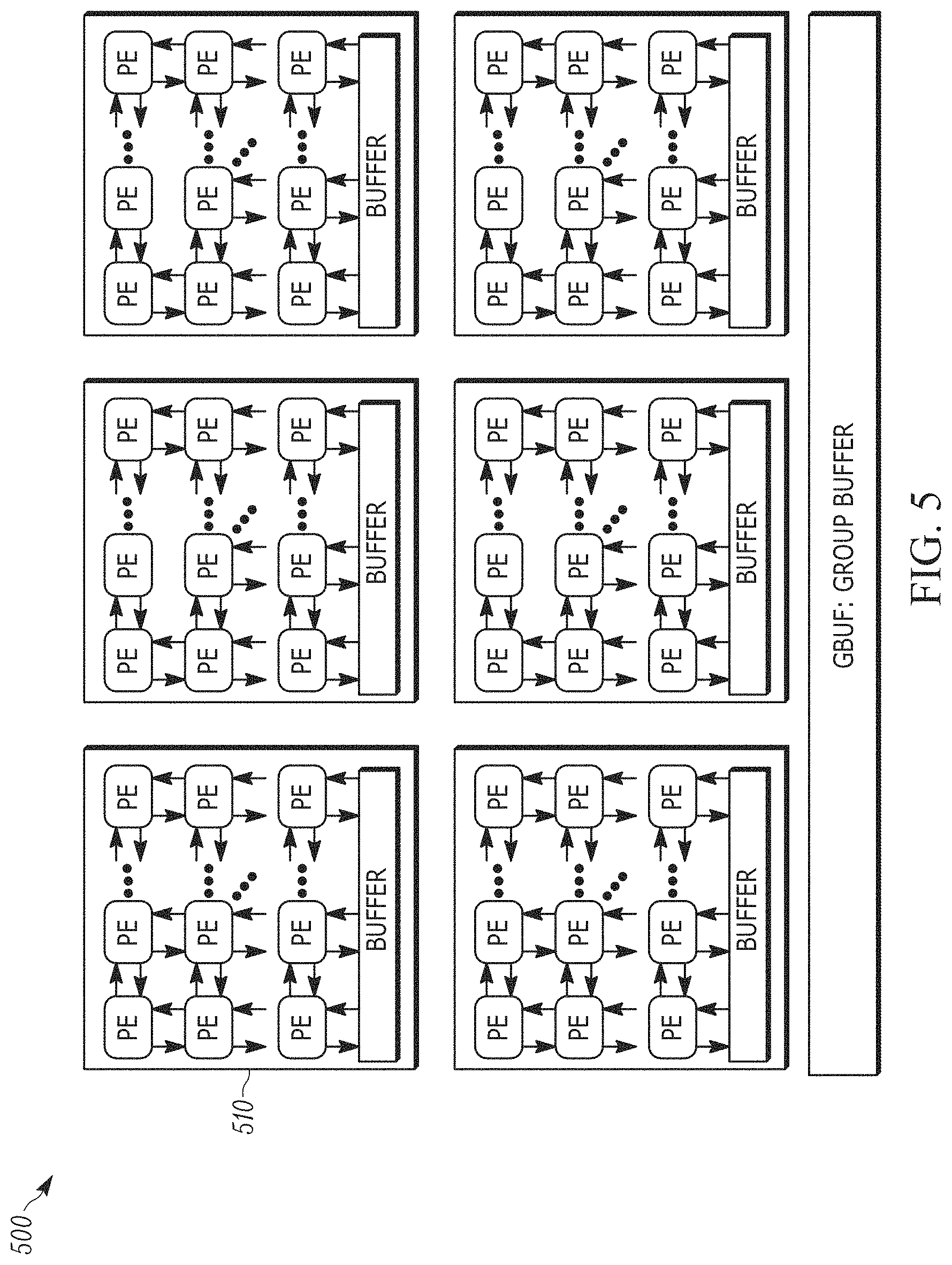
[0098] Thus, a homogeneous accelerator architecture 500 of FIG. 5 would overprovision resources for the different types of operations using a homogeneous set or array 510 of Processing Engines (PEs), and more importantly, (2) would be unable to exploit the algorithmic characteristics of reduced precision from quantization and high sparsity in back-propagated gradients. Therefore, heterogeneity is important to maximize the potential performance benefits using the limited pool of resources on a FPGA die. Motivated by the above insight, a heterogeneous architecture for accelerating quantized training has been designed.
[0099] The present design utilizes a template architecture that is both scalable--to maximally utilize the FPGA's on-chip resources, and customizable--to adapt to the precision requirements of the quantized DNN being trained.
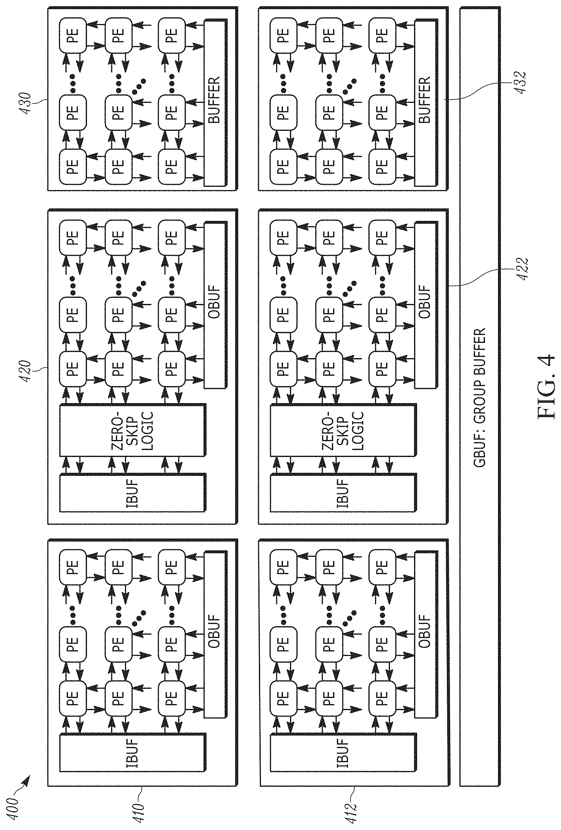
[0100] This heterogenous architecture 400, as shown in FIG. 4, includes three distinct types of computational blocks 410, 420, and 430 that are specialized for the different types of operations for training quantized DNNs. A Dense Quantized Array 410, 412 (DQ-array), which is a systolic array (e.g., 16.times.16 systolic array) of low bit width multiply-accumulate computation units that are labeled as processing engines (PEs) in one example, includes an input buffer, an output buffer, and the PEs.
[0101] A mixed precision zero skipping array 420, 422 (MPZS-array), which is a systolic array (e.g., 16.times.16 systolic array) of mixed-precision multiply-accumulate computation units that are labeled as processing engines (PEs), includes an input buffer, zero skip logic, an output buffer, and PEs.
[0102] Array 430, 432, which is an array (e.g., 4.times.4 array) of floating-point processing engines (PEs), includes a buffer and the PEs. The arrays 410 and 420 are specialized for the highly parallel multiply-add operations in the forward and backward phases of DNNs, while the array 430 is a more general purpose array that can be programmed to either compute element-wise data transformations necessary for quantized training.
[0103] While FPGAs run at a much lower frequency than contemporary processors like CPUs or GPUs, the FPGAs offset the lower frequency by offering high degrees of parallelism for the accelerator. Feeding data to the large number of compute units in the FPGA within the FPGA's limited off-chip bandwidth is challenging, especially due to large memory footprint of DNNs. Fortunately, DNNs have a large degree of data reuse. To utilize the data-reuse for training quantized DNNs, the present design uses a three level memory hierarchy: global, cluster, and local memory (e.g., global-uram, cluster-bram, and local-bram). Unlike caches in CPUs or GPUs, the memory at each level of the hierarchy is controlled by software, making it a scratchpad memory. Using the on-chip memory as scratchpads takes away the burden of prefetching and evicting from the hardware and places it on the software. This enables layer-specific compiler optimizations that take advantage of data-reuse within layers of the quantized DNN.
[0104] The present application will now describe the microarchitecture of the heterogenous architecture 400, and an algorithm for optimizing the sizes of the three types of arrays to maximize performance.
[0105] As previously described herein, the runtime characteristics for the forward and backward phases of quantized training differ significantly. To this end, the present heterogenous architecture uses a MPZS-array that exploits the dual characteristics of high sparsity for the high precision gradients for zero-skipping in the backward phase, and uses a dense quantized execution for the forward phase. The basic building block for the MPZS-array is the CU, which is a bit-flexible compute unit, described below.
[0106] FIG. 6 illustrates the design of a compute unit in accordance with one embodiment. The CU 600 includes n quantized mixed precision multipliers (e.g., 610-613), each of which can multiply up to m-bit operands. While m depends on the minimum precision required by the MAC operations in convolution/fully-connected layers, n depends on the ratio of precision.sub.max/precision.sub.min. The outputs of the n quantized multipliers are added to produce an output 690. The CU supports a flexible range of precision for the floating point or fixed point inputs 601-608 (e.g., floating point 32 bit 601, fixed point 2 bit 602, floating point 32 bit 603, fixed point 2 bit 604, floating point 32 bit 605, fixed point 2 bit 606, floating point 32 bit 607, fixed point 2 bit 608)--activations in the forward phase and the gradients in the backward phase. At the lowest precision mode, the n quantized multipliers in a CU perform n independent multiplications. At the highest precision mode, the n quantized multipliers together multiply a single n.times.m-bit operand with a m-bit operand. In this example, a MPZS array uses a 2D systolic array of 16.times.16 CUs.
[0107] In the dense forward execution mode, each compute unit in the MPZS array performs multiple multiply-add operations for quantized activations and weights in the forward phase of training. The partial results generated by different quantized multipliers are added together to produce a single output.
[0108] As discussed, the gradients in the backward phase for DNNs have high sparsity (e.g., up to 99%). A naive first approach for obtaining performance for such a high degree of sparsity is to serialize the MAC operations using a single row of the systolic array. Such an approach has two drawbacks: (1) each row would require its own single-precision floating point accumulator which would increase the resource cost (FPGA LUT/DSP) per row; and (2) limited parallelism due to a single row.
[0109] A second approach is to use multiple rows in the systolic array, which increases parallelism. Further, outputs within each column of the systolic array can be accumulated in a single floating-point accumulator. The drawback of the second approach is that it enforces synchronization between different rows of the systolic array. That is, each row waits for all the other rows to finish computing the current output before moving on to the next output. Prior work uses the second approach to improve inference performance when the sparsity for activations is between 45-60%. The present design on the other hand aims to exploit the considerably higher sparsity present in the gradients of the backward phase of quantized DNN training. Due to the high sparsity in the gradients for the backward phase, synchronization between different rows of the systolic array would significantly limit the performance benefits from zero-skipping.
[0110] The present design identifies two limitations of the above technique when applied to highly-sparse gradients. The fundamental assumption here is that the compute units in each column synchronize and operate on a single sparse-vector. Therefore, for the first limitation, each row stalls for all the other rows to finish operating on their own sub-vectors before proceeding to the next sparse-vector; which will limit the potential benefits from zero-skipping due to the high-sparsity in gradients.
[0111] For the second limitation, when reading one sparse sub-vector at a time from the memory (e.g., BRAM), the non-zero detect logic will stall when there are no non-zero values in the sub-vector. Assuming a 95% sparsity in gradients, the probability of all zeros in a sub-vector (assuming independent and identical distribution) is 44%.
[0112] To overcome the above second limitation, the present design utilizes a novel low-overhead desynchronized encoding for zero-skipping as illustrated in a multi-lane adder logic 700 of FIG. 7. This encoding uses a desynchronization-tag or d-tag 706 to remove synchronization between rows of a MPZS-array. MPZS-array encodes the non-zero values as value 702, offset 704, and d-tag pair 706. The d-tag 706 specifies the identification (ID) of the sparse-vector that each row operates on. To take advantage of the proposed desynchronized encoding in MPZS-array, the present design uses two tag-lanes 712 and 714 within each column. The compute units in each column share tag-lanes. Within each column, compute units forward their results to one of the tag-lanes using the LSB of the d-tag. When the select logic 730 determines that the tag for the current row matches the previous row's tag for either the odd or even tag-lanes, the values are added together and forwarded to the next row. When the tags do not match, the results are stored locally.
[0113] To overcome the first limitation, the present design decomposes the non-zero detection logic 800 of FIG. 8 into two different modules: (1) zero-detector logic 810, and (2) non-zero selector 820. The zero-detector logic includes a series of comparators that generate a bit-vector that corresponds to using a single bit for each bit of the sub-vector (e.g., 16 bit wide sub-vector). Each bit in the bit-vector specifies if the corresponding value in the sub-vector is zero (low) or non-zero (high). When all bits in the bit-vector are low, the sub-vector is skipped entirely. Otherwise, the sub-vector is pushed to a FIFO queue 830, along with its bit-vector and a d-tag for identifying the input ID. The non-zero selector then pops the FIFO queue to read only those sub-vectors that have some non-zero values. The non-zero selector then selects the first non-zero value and the corresponding offset to produce a (value, offset, tag) pair. Using desynchronization and sub-vector skipping, the present design improves the performance of MPZS-array when sparsity is high.
[0114] While these two techniques improve performance, these techniques also increase the consumption of FPGA's LUT resources. As discussed herein, the resource overhead of sparsity outweighs the benefits from zero-skipping in the forward phase that uses low bit width activations for quantized DNNs. Therefore, the MPZS-array utilizes a dense execution for the forward phase of quantized DNN training, as described below.
[0115] The present design uses a template architecture to implement the MPZS-array on FPGA. The precision for the multiply-add operations can be modified according to the needs of the quantized DNN.
[0116] The following section discusses the scheduling of operations for quantized training across multiple MPZS-arrays. In order to parallelize the operations for training a quantized DNN across multiple MPZS-arrays, the present design splits the computations in each operation into tiles. For most operations required for training quantized DNNs, the total amount of data is often much larger than the limited on-chip memory available on the FPGA. Therefore, splitting the computations into tiles are necessary to fit the data into on-chip memory.
[0117] FIG. 9 illustrates scheduling operations across multiple MPZS-arrays in accordance with one embodiment. To maximize the performance of the MPZS architecture, the present design uses three types of tiling and expresses the task of determining the tile sizes as a constrained optimization problem. The three types of tilings correspond to three levels of memory hierarchy in the MPZS architecture and the sizes of each level of memory hierarchy serves the constraints for optimizing the tile sizes. The present design uses a simple fully-connected layer in FIG. 9 as an example to explain the scheduling of operations 910, 920, 930, and 940. The fully-connected layer from the FIG. 9 can be expressed as a matrix multiplication as follows.
output(B.times.Cout)=input (B.times.Cin).times.weights (Cin.times.Cout) (2)
[0118] FIG. 9 shows how the operations in a fully-connected layer are split into tiles for each level of memory hierarchy including global memory tile (e.g., URAM tile) at operation 910 and cluster memory tile (e.g., BRAM tile) at operation 930. Using a larger tile size for each level of hierarchy increases the data reuse at that level of hierarchy at operation 940. The tile sizes are constrained by the capacity of memory at that level of hierarchy.
[0119] Next, an overview of a DNN workflow 1000 is illustrated in FIG. 10 in accordance with one embodiment. The DNN workflow begins with a programmer defining a Dataflow Graph (DFG) of the DNN using a high-level API. This API allows the programmer to specify the precision for each operation in the DNN. As shown in the FIG. 10, this workflow includes four operations: (1010) a dataflow analysis operation to analyze the resource requirements for the dataflow graph, (1020) a resource partitioning operation to analytically split the FPGA's resources, (1030) a cycle-accurate scheduling operation to obtain cycle counts, and (1040) a builder operation to generate a synthesizable accelerator using the optimal resource breakdown from operation 1030. Below, we describe the four operations in detail.
[0120] For static analysis, the first operation 1010 of the workflow includes analyzing the type of computational resources required by the DNN model. This operation 1010a includes the dataflow analyzer component iterating over the nodes of the dataflow graph of the DNN and generates a list of pairs (e.g., operation type, precision, operation count) for the forward and backward passes of training. In one example, the operation type is a type of scalar operation (e.g., multiply, add, etc), the precision field is a tuple of the data-types required by the operands (e.g., fixed-point, floating-point, or power-of-2), and the operation count field describes the number of scalar operations. Next, the dataflow analyzer generates the highest and lowest precision required for the forward pass and repeats the same for the backward pass. Determining the range of precision requirements is essential for estimating the resources required for compute units in the FPGA (e.g., LUTs, DSPs, and Flip-Flops).
[0121] While static analysis determines the static utilization of the FPGA's resources, runtime analysis is essential to estimate the dynamic utilization considering that a large number of multiply-add operations in a DNN are ineffectual due to one of the operands being zero. At operation 1010b, the dataflow analyzer performs runtime analysis by sampling the data propagated in the forward and backward passes of the dataflow graph for numerous iterations using a user-specified batch-size of inputs. Next, the dataflow analysis calculates the proportion of zero-valued data in sampled data. Using the information generated by the static and runtime analysis in the dataflow analysis operation, the resource partitioning component divides the FPGA's resources as follows at operation 1020.
[0122] The resource partitioner component of the workflow uses an analytical model to obtain the optimal breakdown of the FPGA's resources for forward and backward passes. Since most operations in a DNN are Multiply-Accumulate (MAC) operations, the resource partitioner only considers the MAC operations for the analytical model. For a given pair of (precision.sub.fwd, ops.sub.fwd) and (precision.sub.bwd, ops.sub.fwd) for the forward and backward passes of training, the resource partitioner generates the optimal breakdown (p, 1-p) of FPGA's resources for executing forward and backward passes, respectively.
alu.sub.fwd=p.times.resource.sub.total/resource.sub.fwd (3a)
alu.sub.bwd=(1-p).times.resource.sub.total/resource.sub.bwd (3b)
[0123] Where resource.sub.fwd and resource.sub.bwd are obtained from synthesizing compute units with precision.sub.fwd and precision.sub.bwd, respectively. Next, the resource partitioning component optimizes the ideal number of cycles required by the forward and backward operations given by the following equation:
Cycles.sub.total=ops.sub.fwd.times.nz.sub.fwd/(alu.sub.fwd+alu.sub.bwd)+- (ops.sub.bwd.times.nz.sub.bwd)/alu.sub.bwd (4)
[0124] Using equations [3b] and [3b], equation [4] solved quadratically to get the optimal partitioning p as follows.
Minimize p cycles.sub.total(p),p.di-elect cons.[0,1) (5)
p=-c+1/c.times.r-1+square root ((c+1)2/(c.times.r-1)2-c-r/r.times.(c.times.r-1) (6)
where c=ops.sub.bwd.times.nz.sub.bwd/(op.sub.fwd.times.nz.sub.bwd) (7)
r=resource.sub.bwd/resource.sub.fwd-1 (8)
[0125] Here, the c term is the ratio of non-zero computations in the backward pass to the non-zero computations in the forward pass, and r term is the one minus the ratio of resources required for the backward pass to the resources required by the forward pass. While computing the value of r requires static information, computing c requires both static and dynamic information.
[0126] The value of p obtained from equation [6] is the optimal breakdown of the FPGA's resources assuming no under-utilization of resources due to memory accesses. In reality, however, even quantized DNNs have a large memory footprint and hence performance of the generated FPGA accelerator depends both on the breakdown of the FPGA's resources and the organization of on-chip memory. Nevertheless, the value of p obtained from equation [6] serves as a good initial solution for optimizing the breakdown of the FPGA's resources.
[0127] Next, the scheduler component evaluates the solution provided by the resource partitioner. The scheduler is the third component of the workflow which evaluates the quality of the solution generated by the resource partitioner. The present design uses an architectural vs cycle-accurate simulation model for determining the quality of the partitioning solution. First, the simulator component divides the FPGA's LUT and DSP resources into 16.times.16 systolic arrays for the forward and backward passes using the p obtained from the resource partitioner.
[0128] Next, the simulator evenly divides the FPGA's memory (e.g., URAM and BRAM) resources for each systolic array. The architecture of the present design uses a 2 level hierarchy for organizing the on-chip memory, as discussed above. Finally, using the number of forward and backward systolic arrays along with the memory organization, the simulator component performs cycle-accurate simulation. The simulation model accounts for limited bandwidth and latency for communication over both PCIe and the off-chip DRAMs. The scheduler generates the cycle counts for DQ-array and MPZS-array. Using the cycle-counts, the scheduler updates the compute ratio c defined in Equation [7] as follows.
cnext=cyclesDQ-array/cyclesMPZS-array (9)
[0129] The scheduler then feeds back the updated compute ratio to the resource partitioner. Algorithm 1 summarizes the tasks of the Dataflow Analyzer, Resource Partitioner, and Scheduler. Since the present design aims to flexibly support a wide range of quantized training algorithms, it uses a template architecture to accelerate a wide range of quantized DNNs. The first three components generate an optimized set of parameters for the template architecture along with an optimized execution schedule. The last component, the builder generates a synthesizable accelerator using both the optimized set of architectural parameter and execution schedule.
TABLE-US-00001 Algorithm 1: heterogenous resource partitioning Inputs : D: DFG of the quantized DNN resource.sub.total : FPGA's total resources Output : p: Optimal breakdown of resources for DQ-array schedule: Schedule of operations for the optimized p arg min : cycles.sub.total : The total execution cycles forone training iteration Function AnalyzeDFG(D) //Static Analysis //Number of operations in forward/backward ops.sub.fwd, ops.sub.bwd <- D // Tuple of precision per layer precision.sub.fwd .sub.<- ops.sub.fwd precision.sub.bwd .sub.<- ops.sub.bwd LUT/DSP resources for forward operations resource.sub.fwd .sub.<- precision.sub.fwd resource.sub.bwd .sub.<- precision.sub.bwd Runtime analysis nz.sub.fwd, nz.sub.bwd .sub.<- execute(D) Obtain c and r c <- opbwd x nzbwd / opf wd x nz f wd r <- resourcebwd/resource f wd -1 return c, r end Function Partition(c, r) return p = - c+1 / cxr-1 +r squareroot ((c+1)2/(cxr-1)2 - c-r /rx(cxr-1)) end Function Schedule(D, p) // Schedule and estimate cycles for forward/backward phase cycles f wd, cyclesbwd <- Model(D, p) return cycles f wd, cyclesbwd end Initialize c, r AnalyzeDFG(D) cycles f wd, cyclesbwd Schedule(D, p) cnext <- cyclesbwd / cycles f wd // Refine the partitioning Initialize cnext <- - infinity Do p < - Partition(c, r) cycles f wd, cyclesbwd < - Schedule(D, p) cnext < - cyclesbwd / cycles f wd while abs value( c-cnext) > epsilon;
TABLE-US-00002 # of Batch # of Ops param- Benchmark Quantization Dataset Size (per-batch) eters AlexNet-D DoReFa-Net ImageNet 128 8,256 Mops 62M SVHN-D DoReFa-Net SVHN 128 342 Mops 62M AlexNet-D QNN ImageNet 512 2067 Mops 50M Cifar-10-Q QNN Cifar-10 50 1,844 Mops 12M SVHN-Q QNN SVHN 200 469 Mops 5M Google- QNN ImageNet 64 4777 Mops 56M Net-Q AlexNet-W WRPN ImageNet 54 31,503 Mops 108M ResNet-W WRPN ImageNet 64 12025 Mops 23M
[0130] Table I shows the evaluated benchmarks, their datasets, number of operations, model size, and final accuracy. The postfix -W, -Q, -D refer to quantization techniques proposed by different prior approaches that use uniform quantization using fixed-point representation for activations and weights but use different quantization strategies for gradients. For gradients, DoReFa-Net uses fixed-point quantization with added gaussian noise, QNN uses logarithmic quantization using a power-of-2 data representation, and WRPN uses floating-point. Benchmarks ResNet-34-W, GoogleNet-Q, AlexNet-Q, AlexNet-W, AlexNet-D are image classification models trained on the Imagenet 2012 dataset. Benchmarks SVHN-W and SVHN-Q are optical character recognition models based on the SVHN dataset. Unlike inference, the quality of the trained model depends significantly on the batch size. Therefore, the same batch sizes reported in these prior approaches is used for both GPUs and the heterogenous architecture of the present design. Furthermore, the three benchmarks use stochastic noise to speed-up convergence. Across all the benchmarks, both performance and power consumption are measured for a FPGA platform and a GPU platform for 10,000 training iterations and present the average. For both GPU and FPGA implementations, the host CPU is used as the parameter server.
[0131] A FPGA platform includes 6840 DSPs, 1182K LUTs, 33.7 MB URAM, 8.4 MB BRAMs, 42 W TDP, 200 MHz frequency, and 16 nm technology node. A GPU platform has 3584 cores, 12 GB memory, 250 W TDP, 1531 MHz frequency, and 16 nm technology node.
[0132] FIGS. 11 and 12 illustrate performance of the GPU platform in comparison to different variations of the present design as implemented in the FPGA platform.
[0133] The present design provides an alternative solution for GPUs, by leveraging the inherent characteristic of quantized deep learning and introducing heterogeneous accelerator architecture for FPGAs. As such, this design exists at the intersection of (a) quantization for deep learning, (b) acceleration for quantized deep learning, (c) acceleration for ML training, (d) heterogeneous architecture, and (e) exploitation of sparsity in deep learning.
[0134] FIG. 13 illustrates the schematic diagram of data processing system 1300 according to an embodiment of the present invention. Data processing system 1300 includes I/O processing unit 1310 and general purpose instruction-based processor 1320. In an embodiment, general purpose instruction-based processor 1320 may include a general purpose core or multiple general purpose cores. A general purpose core is not tied to or integrated with any particular algorithm. In an alternative embodiment, general purpose instruction-based processor 1320 may be a specialized core. I/O processing unit 1310 may include an accelerator 1311 (e.g., in-line accelerator, offload accelerator for offloading processing from another computing resource, accelerator with heterogenous architecture for DNN training, etc.) for implementing embodiments as described herein. In-line accelerators are a special class of accelerators that may be used for I/O intensive applications. Accelerator 1311 and general purpose instruction-based processor may or may not be on a same chip. Accelerator 1311 is coupled to I/O interface 1312. Considering the type of input interface or input data, in one embodiment, the accelerator 1311 may receive any type of network packets from a network 1330 and an input network interface card (NIC). In another embodiment, the accelerator maybe receiving raw images or videos from the input cameras. In an embodiment, accelerator 1311 may also receive voice data from an input voice sensor device.
[0135] In an embodiment, accelerator 1311 partially performs the computation associated with the input data elements and transfers the control to other accelerators or the main general purpose instruction-based processor in the system to complete the processing. The term "computation" as used herein may refer to any computer task processing including, but not limited to, any of arithmetic/logic operations, memory operations, I/O operations, and offloading part of the computation to other elements of the system such as general purpose instruction-based processors and accelerators. Accelerator 1311 may transfer the control to general purpose instruction-based processor 1320 to complete the computation.
[0136] In an embodiment, accelerator 1311 may be implemented using any device known to be used as accelerator, including but not limited to field-programmable gate array (FPGA), Coarse-Grained Reconfigurable Architecture (CGRA), general-purpose computing on graphics processing unit (GPGPU), many light-weight cores (MLWC), network general purpose instruction-based processor, I/O general purpose instruction-based processor, and application-specific integrated circuit (ASIC). In an embodiment, I/O interface 1312 may provide connectivity to other interfaces that may be used in networks, storages, cameras, or other user interface devices. I/O interface 1312 may include receive first in first out (FIFO) storage 1313 and transmit FIFO storage 1314. FIFO storages 1313 and 1314 may be implemented using SRAM, flip-flops, latches or any other suitable form of storage. The input packets are fed to the accelerator through receive FIFO storage 1313 and the generated packets are sent over the network by the accelerator and/or general purpose instruction-based processor through transmit FIFO storage 1314.
[0137] In an embodiment, I/O processing unit 1310 may be Network Interface Card (NIC). In an embodiment of the invention, accelerator 1311 is part of the NIC. In an embodiment, the NIC is on the same chip as general purpose instruction-based processor 1320. In an alternative embodiment, the NIC 1310 is on a separate chip coupled to general purpose instruction-based processor 1320. In an embodiment, the NIC-based accelerator receives an incoming packet, as input data elements through I/O interface 1312, processes the packet and generates the response packet(s) without involving general purpose instruction-based processor 1320. Only when accelerator 1311 cannot handle the input packet by itself, the packet is transferred to general purpose instruction-based processor 1320. In an embodiment, accelerator 1311 communicates with other I/O interfaces, for example, storage elements through direct memory access (DMA) to retrieve data without involving general purpose instruction-based processor 1320.
[0138] Accelerator 1311 and the general purpose instruction-based processor 1320 are coupled to shared memory 1343 through private cache memories 1341 and 1342 respectively. In an embodiment, shared memory 1343 is a coherent memory system. The coherent memory system may be implemented as shared cache. In an embodiment, the coherent memory system is implemented using multiples caches with coherency protocol in front of a higher capacity memory such as a DRAM.
[0139] In an embodiment, the transfer of data between different layers of accelerations may be done through dedicated channels directly between accelerator 1311 and processor 1320. In an embodiment, when the execution exits the last acceleration layer by accelerator 1311, the control will be transferred to the general-purpose core 1320.
[0140] Processing data by forming two paths of computations on accelerators and general purpose instruction-based processors (or multiple paths of computation when there are multiple acceleration layers) have many other applications apart from low-level network applications. For example, most emerging big-data applications in data centers have been moving toward scale-out architectures, a technology for scaling the processing power, memory capacity and bandwidth, as well as persistent storage capacity and bandwidth. These scale-out architectures are highly network-intensive. Therefore, they can benefit from acceleration. These applications, however, have a dynamic nature requiring frequent changes and modifications. Therefore, it is highly beneficial to automate the process of splitting an application into a fast-path that can be executed by an accelerator with subgraph templates and a slow-path that can be executed by a general purpose instruction-based processor as disclosed herein.
[0141] While embodiments of the invention are shown as two accelerated and general-purpose layers throughout this document, it is appreciated by one skilled in the art that the invention can be implemented to include multiple layers of computation with different levels of acceleration and generality. For example, a FPGA accelerator can backed by a many-core hardware. In an embodiment, the many-core hardware can be backed by a general purpose instruction-based processor.
[0142] Referring to FIG. 14, in an embodiment of invention, a multi-layer system 1000 is formed by a first accelerator 1011.sub.1 (e.g., in-line accelerator, offload accelerator for offloading processing from another computing resource, accelerator with heterogenous architecture for DNN training, or both) and several other accelerators 1011.sub.n (e.g., in-line accelerator, offload accelerator for offloading processing from another computing resource, accelerator with heterogenous architecture for DNN training, or both). The multi-layer system 1050 includes several accelerators, each performing a particular level of acceleration. In such a system, execution may begin at a first layer by the first accelerator 1011.sub.1. Then, each subsequent layer of acceleration is invoked when the execution exits the layer before it. For example, if the accelerator 1011.sub.1 cannot finish the processing of the input data, the input data and the execution will be transferred to the next acceleration layer, accelerator 1011.sub.2. In an embodiment, the transfer of data between different layers of accelerations may be done through dedicated channels between layers (e.g., 1071.sub.1 to 1071.sub.n). In an embodiment, when the execution exits the last acceleration layer by accelerator 1011.sub.n, the control will be transferred to the general-purpose core 1090.
[0143] FIG. 15 is a diagram of a computer system including a data processing system that utilizes an accelerator according to an embodiment of the invention. Within the computer system 1200 is a set of instructions for causing the machine to perform any one or more of the methodologies discussed herein including accelerating machine learning operations. In alternative embodiments, the machine may be connected (e.g., networked) to other machines in a LAN, an intranet, an extranet, or the Internet. The machine can operate in the capacity of a server or a client in a client-server network environment, or as a peer machine in a peer-to-peer (or distributed) network environment, the machine can also operate in the capacity of a web appliance, a server, a network router, switch or bridge, event producer, distributed node, centralized system, or any machine capable of executing a set of instructions (sequential or otherwise) that specify actions to be taken by that machine. Further, while only a single machine is illustrated, the term "machine" shall also be taken to include any collection of machines (e.g., computers) that individually or jointly execute a set (or multiple sets) of instructions to perform any one or more of the methodologies discussed herein.
[0144] Data processing system 1202, as disclosed above, includes a general purpose instruction-based processor 1227 and an accelerator 1226 (e.g., in-line accelerator, offload accelerator for offloading processing from another computing resource, accelerator with heterogenous architecture for DNN training, etc.). The general purpose instruction-based processor may be one or more general purpose instruction-based processors or processing devices (e.g., microprocessor, central processing unit, or the like). More particularly, data processing system 1202 may be a complex instruction set computing (CISC) microprocessor, reduced instruction set computing (RISC) microprocessor, very long instruction word (VLIW) microprocessor, general purpose instruction-based processor implementing other instruction sets, or general purpose instruction-based processors implementing a combination of instruction sets. The accelerator may be one or more special-purpose processing devices such as an application specific integrated circuit (ASIC), a field programmable gate array (FPGA), a digital signal general purpose instruction-based processor (DSP), network general purpose instruction-based processor, many light-weight cores (MLWC) or the like. Data processing system 1202 is configured to implement the data processing system for performing the operations and steps discussed herein.
[0145] The exemplary computer system 1200 includes a data processing system 1202, a main memory 1204 (e.g., read-only memory (ROM), flash memory, dynamic random access memory (DRAM) such as synchronous DRAM (SDRAM) or DRAM (RDRAM), etc.), a static memory 1206 (e.g., flash memory, static random access memory (SRAM), etc.), and a data storage device 1216 (e.g., a secondary memory unit in the form of a drive unit, which may include fixed or removable computer-readable storage medium), which communicate with each other via a bus 1208. The storage units disclosed in computer system 1200 may be configured to implement the data storing mechanisms for performing the operations and steps discussed herein. Memory 1206 can store code and/or data for use by processor 1227 or accelerator 1226. Memory 1206 include a memory hierarchy that can be implemented using any combination of RAM (e.g., SRAM, DRAM, DDRAM), ROM, FLASH, magnetic and/or optical storage devices. Memory may also include a transmission medium for carrying information-bearing signals indicative of computer instructions or data (with or without a carrier wave upon which the signals are modulated).
[0146] Processor 1227 and accelerator 1226 execute various software components stored in memory 1204 to perform various functions for system 1200. Furthermore, memory 1206 may store additional modules and data structures not described above.
[0147] Operating system 1205a includes various procedures, sets of instructions, software components and/or drivers for controlling and managing general system tasks and facilitates communication between various hardware and software components. A compiler is a computer program (or set of programs) that transform source code written in a programming language into another computer language (e.g., target language, object code). A communication module 1205c provides communication with other devices utilizing the network interface device 1222 or RF transceiver 1224.
[0148] The computer system 1200 may further include a network interface device 1222. In an alternative embodiment, the data processing system disclose is integrated into the network interface device 1222 as disclosed herein. The computer system 1200 also may include a video display unit 1210 (e.g., a liquid crystal display (LCD), LED, or a cathode ray tube (CRT)) connected to the computer system through a graphics port and graphics chipset, an input device 1212 (e.g., a keyboard, a mouse), a camera 1214, and a Graphic User Interface (GUI) device 1220 (e.g., a touch-screen with input & output functionality).
[0149] The computer system 1200 may further include a RF transceiver 1224 provides frequency shifting, converting received RF signals to baseband and converting baseband transmit signals to RF. In some descriptions a radio transceiver or RF transceiver may be understood to include other signal processing functionality such as modulation/demodulation, coding/decoding, interleaving/de-interleaving, spreading/dispreading, inverse fast Fourier transforming (IFFT)/fast Fourier transforming (FFT), cyclic prefix appending/removal, and other signal processing functions.
[0150] The Data Storage Device 1216 may include a machine-readable storage medium (or more specifically a computer-readable storage medium) on which is stored one or more sets of instructions embodying any one or more of the methodologies or functions described herein. Disclosed data storing mechanism may be implemented, completely or at least partially, within the main memory 1204 and/or within the data processing system 1202 by the computer system 1200, the main memory 1204 and the data processing system 1202 also constituting machine-readable storage media.
[0151] In one example, the computer system 1200 is an autonomous vehicle that may be connected (e.g., networked) to other machines or other autonomous vehicles in a LAN, WAN, or any network. The autonomous vehicle can be a distributed system that includes many computers networked within the vehicle. The autonomous vehicle can transmit communications (e.g., across the Internet, any wireless communication) to indicate current conditions (e.g., an alarm collision condition indicates close proximity to another vehicle or object, a collision condition indicates that a collision has occurred with another vehicle or object, etc.). The autonomous vehicle can operate in the capacity of a server or a client in a client-server network environment, or as a peer machine in a peer-to-peer (or distributed) network environment. The storage units disclosed in computer system 1200 may be configured to implement data storing mechanisms for performing the operations of autonomous vehicles.
[0152] The computer system 1200 also includes sensor system 1214 and mechanical control systems 1207 (e.g., motors, driving wheel control, brake control, throttle control, etc.). The processing system 1202 executes software instructions to perform different features and functionality (e.g., driving decisions) and provide a graphical user interface 1220 for an occupant of the vehicle. The processing system 1202 performs the different features and functionality for autonomous operation of the vehicle based at least partially on receiving input from the sensor system 1214 that includes laser sensors, cameras, radar, GPS, and additional sensors. The processing system 1202 may be an electronic control unit for the vehicle.
[0153] Neural Networks can tolerate a reduction in precision for operations in Neural Network inference and in the forward propagation phase of Neural Network training, while retaining classification accuracy. The potential benefits from using either quantized data representation or block floating-point representation are two-folds: (1) using quantized or block floating-point reduces the memory storage requirements for the data in a Neural Network model; and (2) compute units for reduced precision require significantly less energy and area compared to floating-point compute units.
[0154] However, the precision required for different data types and operations for Neural Network training can vary for both inference and training. Further, the operations in the backward propagation phase of Neural Network training may require higher precision compared to the forward propagation phase of Neural Network training.
[0155] This present design identifies that the key challenge for exploiting the aforementioned benefits is that the precision for different operands in a reduced-precision NN model can vary to retain the same accuracy as the floating-point NN model. Traditional architectures, including architectures for CPUs/GPUs, and even hardware accelerators that are FPGA-based or ASICs proposed by prior works, are limited to homogeneous precision in the operations that they can perform. Thus, when executing a NN model that requires a mixture of different precision requirements--such as floating-point and quantized data representation--traditional architectures first need to convert all the quantities to floating-point precision to perform computations.
[0156] Below, we first present a homogeneous-precision systolic-array architecture as a reference design.
[0157] FIG. 16 shows the details of the specialized circuit 1700 for accelerating neural networks training and inference in prior art. The specialized circuit in FIG. 16 includes of one or more circuits 1701 that are specialized for one or more computations in neural networks. For example, the systolic array circuit 1701 shown in FIG. 16 is specialized for the convolution and matrix-multiplication operations in neural networks.
[0158] The systolic array circuit 1701 further includes of (1) a plurality of CUs 1800 that perform the operations in the plurality of layers in neural network training and inference, (2) a buffer IBUF 1704 to store inputs and (3) a buffer OBUF 1705 to store intermediate results when executing the operations for the multi-dimensional arrays of data in neural network.
[0159] The circuit 1700 may further contain a GBUF 1710 that enables the multiple instances of circuit 1701 to share data.
[0160] The CUs 1800 in FIG. 16 are organized as a 2-dimensional grid, with a plurality of rows 1702 and a plurality of columns 1703.
[0161] The buffer IBUF 1704 feeds data to the CU 1800 on the first column (the left most column), as shown in FIG. 16. The results from the CUs 1800 in each column of the systolic array are accumulated in an accumulator circuit and the stored in the OBUF 1705.
[0162] Each CU 1800, can perform multiply-add operations, with one operand from the CU 1800 in the previous column (the CU 1800 on the left), with one operand from the CU 1800's private buffer called WBUF 1803 to generate a product. The product is then added with the result from the CU 1800 in the previous row (the CU 1800 on the top) and sent to the CU 1800 in the next row (the CU 1800 on the bottom). Thus, data is shared between CUs 1800 in a row and the output from CUs 1800 in a column are accumulated and sent downwards.
[0163] FIG. 17 shows the details of the CU 1800 in the systolic array circuit. The CU 1800 multiplies one value from either the previous CU 1800 (the CU 1800 on the left) or from the IBUF 1704, with one value from the CU 1800's private buffer WBUF 1803. The resulting product is added with the results from the previous CU 1800. The resulting sum is then forwarded to the CU 1800 in the next row (CU 1800 on the bottom).
[0164] In some implementations, an accumulator circuit 1707 may perform additional operations (max, min, multiplication, etc) required for different layers of the neural network (like pooling, activation, etc).
[0165] When the size of the data required for inputs and the outputs for layers of the neural network is larger than the capacity of the on-chip buffers (IBUF 1704, WBUF 1803, and OBUF 1705), then the data is divided into portions such that size of each portion does not exceed the capacity of on-chip buffers.
[0166] One notable feature of hardware acceleration circuits in prior art is that the precision for multidimensional array inputs for the layers of neural networks is the same. Consequently, the width of the IBUF 1704 and WBUF 1803 buffers are sized according to the precision of the operands supported by the circuit, and the width of the OBUF 1705 is sized according to the precision for the intermediate data. Similarly, the CUs 1800 in the systolic array is designed for the precision supported by the circuit.
[0167] The reference circuit 1700 uses homogeneous precision--all CUs 1800 in the circuit 1700 use the same precision for all operands.
[0168] When using a homogeneous architecture, such as the circuit 1700 presented FIG. 1, all the multidimensional arrays of data that are input the Neural Network operations have to converted to the same precision that is supported by the circuit.
[0169] In FIG. 18 the taxonomy 1900 of the different strategies for heterogeneous precision in the circuit for computations in Neural Network training and inference is illustrated.
[0170] The first classification 1910 for heterogeneous precision circuits for Neural Network training and inference is based on how compute units with different precisions are organized.
[0171] FIG. 19 shows the first method, called coarse-grained heterogeneous precision 1911. The precision for Compute Units (CUs) with different precisions (e.g., 32-bit floating-point, 16-bit floating-point, 32-bit fixed-point, 16-bit fixed-point, 11-bit fixed-point, etc)--2002, 2006, 2010--are grouped together in the same systolic array, while the precision for CUs varies across different systolic arrays--2001, 2005, 2009.
[0172] The width of the buffers 2003 and 2004 are sized according to the precision of the CU 2002; width of the buffers 2007 and 2008 are sized according to the precision of the CU 2006; and width of the buffers 2011 and 2012 are sized according to the precision of the CU 2010.
[0173] Coarse-grained heterogeneity 1911 in precision for CUs enables the accelerator to match groups of operations with different precision requirements to CUs that match the precision required by the neural network and provide the highest efficiency. Thus, coarse-grained heterogeneous precision avoids the costly conversion of the different data representations to a common floating-point data representation necessary for homogeneous-precision architectures.
[0174] The example shown in FIG. 19 illustrates that, if a NN model requires both floating-point and binary precisions for operations, the floating-point operations can execute using the floating-point systolic array (e.g., 2001) and the binary operations execute using a different binary systolic array that supports binary precision (e.g., 2005). Accordingly, the circuits 2001 and 2005 have to be designed to support floating-point and binary precision, respectively.
[0175] Similarly, if a NN model requires multiple different precisions for the different multidimensional arrays of data in the NN, the circuit 2000 can include multiple different systolic arrays, where each individual systolic array supports one or more precision configuration (e.g, floating-point, binary, etc) required by the NN model.
[0176] One application for coarse-grained precision heterogeneity is training for neural networks. Neural network training can be divided into two parts: (1) forward propagation and (2) backward propagation. The forward propagation part of training has higher tolerance to reduced precision as compared to backward propagation part. As such, coarse-grained precision heterogeneity enables the use of specialized compute units that are (1) low-precision for the forward-propagation computations and (2) high-precision for the backward propagation computations.
[0177] FIG. 20 shows the second method, called fine-grained heterogeneous precision 1912. Using fine-grained heterogeneous precision, the precision for the different CUs (2101, 2102, and 2103) within the same systolic array 2100 can vary. Fine-grained heterogeneous precision 1912 enables the precision for operations in the Neural Network to vary within groups of operations and still avoid the costly conversions to a common data representation that is necessary for both homogeneous-precision architectures 1700 in prior art and coarse-grained heterogeneous precision circuit 2000. Furthermore, the width of the WBUF within each CU (2101, 2102, and 2103) are sized according to the precision supported by that CU.
[0178] One application for fine-grained precision heterogeneity 1912 is when generating fully-customized ASICs that are specialized for the operations in a singular neural network. Fine-grained precision heterogeneity for fully-customized ASICs enables the precision for each CU in the hardware to be optimized for the specific neural network being accelerated.
[0179] Further, fine-grained precision heterogeneity 1912 enables individual values in the multidimensional arrays of data in Neural Networks to use different precision. In one example, a single array of data can include individual scalar values with floating-point precision, binary-precision, 8-bit fixed-point precision, etc.
[0180] The second classification 1901 for heterogeneous precision circuits for Neural Network training and inference is based on the precision of the multidimensional arrays of inputs, weights, gradients, and other data in Neural Networks supported by the circuit.
[0181] The first category is symmetric heterogeneous precision 1903, wherein the precision for the different multidimensional arrays of inputs, weights, gradients, and other data in Neural Networks is the same. For instance, the precision for both inputs and weights for a convolution layer in a Neural Network that is supported by the circuit is either floating-point for both inputs and weights, or reduced precision (e.g., 16-bit fixed-point, 8-bit fixed-point, 3-bit fixed-point, etc) for both inputs and weights.
[0182] In one implementation of symmetric heterogeneous precision 1903 circuit, FIG. 21 shows an example of a systolic array 2200 that can operate on two multidimensional arrays of data, with either both multidimensional arrays of data being floating-point 2201 or both multidimensional arrays of data are binary precision 2209. In one example, for a convolution operation in Neural Networks, the 2201 circuit will support 32-bit floating-point precision for both inputs and weights, and the 2209 circuit will support 1-bit binary precision for both inputs and weights.
[0183] Accordingly, the 2202 is designed to perform 32-bit floating-point multiply-add operations, and the buffer IBUF 2203, buffer OBUF 2204, and the buffer WBUF private to the 2202 is designed to supply 32-bit values to the array of CUs. Similarly, the 2210 is designed to perform 1-bit binary multiply-add operations, and the 2211 and the buffer WBUF private to the 2210 is designed to supply 1-bit values to the array of CUs. The buffer OBUF 2212 can be designed to hold either binary precision data, or hold intermediate results with higher precision (eg. 16-bit fixed-point, or 16-bit floating-point, etc) to avoid overflow.
[0184] The second category is asymmetric heterogeneous precision 1902, wherein the precision for the different multidimensional arrays of inputs, weights, gradients, and other data in Neural Network training and inference are different.
[0185] In one implementation of asymmetric heterogeneous precision 1902 circuit, FIG. 22 shows examples of a systolic array 2300 that can operate on two multidimensional arrays of data, with the precision of both multidimensional arrays of data being different.
[0186] In one exemplar implementation, the precision for both inputs and weights for a convolution layer in a Neural Network that is supported by the circuit is floating-point for inputs and binary for weights in circuit 2301; and binary for inputs and 16-bit fixed-point for weights in circuit 2305. Accordingly, the CUs 2302 in circuit 2301 are designed to perform multiplication between individual inputs and weights with floating-point and binary precision, respectively. The buffers 2303 is designed to supply inputs with floating-point precision and the private WBUF in 2302 is designed to supply weights with binary precision. Similarly, the CUs 2306 in circuit 2305 are designed to perform multiplication between individual inputs and weights with binary and binary 16-bit fixed-point precision, respectively. The buffers 2307 is designed to supply inputs with binary precision and the private WBUF in 2306 is designed to supply weights with 16-bit fixed-point precision.
[0187] The third classification 1905 for heterogeneous precision circuits for Neural Network training and inference is based on the programmability offered by the circuit to change the precision supported for the multidimensional arrays of inputs, weights, gradients, and other data for operations in Neural Networks supported by the circuit.
[0188] The first category is flexible precision 1906, wherein the precision for the different multidimensional arrays of inputs, weights, gradients, and other data supported for the operations in Neural Networks can be flexibly changed. A sub-category of flexible precision 1906 is software-configurable flexible precision 1907, wherein the precision for the different multidimensional arrays can be programmed through software at runtime.
[0189] FIG. 23 shows one embodiment of software-configurable flexible precision 1907, which is a circuit 2400 that can match the precision requirements for the multidimensional arrays of data in Neural Network dynamically to execute the various training and inference operations in Neural Networks. Specifically, the circuit 2400 can operate on two multidimensional arrays in Neural Networks and can support both 8-bit fixed-point precision and 4-bit fixed-point precision for the two arrays. The on-chip buffers IBUF 2403 and the WBUF that is private to each CU 2451 are sized appropriately to supply data according to the highest precision (8-bit fixed-point) supported by the circuit.
[0190] Depending on the software configuration, each CU 2450 can perform a multiplication between two individual operands in either a single cycle when the precision is 4-bit for both operands. The shifter 2454, the adder 2456, and the register 2470 allows the CU to perform multiplication when the precision is 8-bit for just one operand over two cycles; or use four cycles when the precision is 8-bit for just both operands.
[0191] In another implementation of circuit 2400, the CU 2450 can include a plurality of multipliers and shifters that can perform 8-bit multiplications in a single cycle and either (1) perform multiple 4-bit operations (2) power-gated to conserve energy for 4-bit.
[0192] Further, the circuit 2400 is just one exemplary implementation of software-programmable heterogeneous precision circuits. Other implementations that can support different precisions (16-bit fixed-point, 12-bit fixed-point, 2-bit fixed-point, floating-point, etc) are possible by using multipliers 2454 and shifters 2455 with appropriate precision.
[0193] A second sub-category of flexible precision 1906 is hardware-configurable flexible precision 1908 is specific to FPGA-based implementation, wherein the precision for the different multidimensional arrays can be programmed through software by reprogramming the FPGA. Reprogramming the either the entire FPGA or partial reconfiguration of a part of the logic in the FPGA enables the ability to switch between different precisions.
[0194] Finally, the last category for flexible precision 1906 is 1909, wherein the precision for the multidimensional arrays of data for Neural Network training and inference cannot be changed. The circuit in prior art 1700 is an example of 1909, where the precision for data is fixed to 32-bit floating-point.
[0195] Built upon our reference design, described in circuits 2000, 2100, 2200, 2300, and 2400, this specification provides exemplary acceleration designs by taking a design choice per each dimension of precision heterogeneity as one embodiment of this specification in FIG. 24. Although the figures illustrate a certain number of blocks (e.g., computation units, computational block, etc.), the present design may include any number of different blocks for different embodiments.
[0196] Circuit 2500 includes of one or more the following two types of circuits: (1) coarse-grained asymmetric heterogeneous precision circuit 2501, (2) coarse-grained asymmetric software-programmable heterogeneous precision circuit 2510. The two circuits, 2501 and 2510, together perform the operations in Neural Network training and inference.
[0197] FIG. 26 shows the data and operations for quantized Neural Network training for a single convolution layer.
[0198] The circuit 2501 is responsible for the CONVF operation 2710 in the forward propagation for neural network training and uses 8-bit precision for inputs 2701 and 4-bit precision for weights 2702. As such, the IBUF 2503 stores the inputs of the Neural Network in 8-bit precision. The data read from IBUF is then shared across all CUs 2502 in a row of the circuit 2501.
[0199] Similar to the CU in FIG. 22, the CU 2502 includes of a private buffer WBUF that stores the weights 2702 in 4-bit precision.
[0200] The intermediate results generated by the CUs 2502 in a column of 2501 require more number of bits compared to the inputs 2701 and weights 2702, and can be adjusted to avoid overflows. The intermediate results generated by circuit 2502 are then accumulated and stored in the OBUF 2504.
[0201] In contrast, circuit 2510 is responsible for the backward propagation operations in Neural Network training and supports floating-point representation for the gradients and both 8-bit and 4-bit precision for the inputs and weights, respectively. Thus, the IBUF 2512 stores the gradients 2751 of the Neural Network in 32-bit floating-point precision. The data read from IBUF is then shared across all CUs in a row of the circuit 2501.
[0202] Similar to the CU in FIG. 22, the CU 2511 includes of a private buffer WBUF that stores the weights 2702 in 4-bit and the inputs 2701 in 8-bit precision. The CU 2600 is further described in FIG. 25.
[0203] FIG. 25 shows the details of the CU 2600, implemented in the asymmetric software-programmable circuit 2510. The CU 2600 includes of a private WBUF 2620 that can store both 8-bit inputs and 4-bit weights in the example. Each entry in WBUF 2620 is 4-bit wide and can either hold an entire value for weights or store either the lower or upper half of inputs.
[0204] In one exemplary implementation, to perform a multiplication between the floating-point value 2601 and 4-bit fixed-point value 2602 read from IBUF 2612, the sign 2603 and mantissa 2605 bits are converted to 2's complement form 2606. The fixed-point multiplier 2607 performs the multiplication and the product is combined with the exponent bits 2604.
[0205] The CU takes a single cycle for multiplying a gradients value with weights, and two cycles for the 8-bit inputs value. The left-shifts the results from the multiplier 2607 by 4-bits when generating the results for the upper 4-bits for the 8-bit inputs value. The left-shifts does not perform any shifting for weights and the lower 4-bits of inputs value.
[0206] The intermediate results 2608 is then added with the results 2609 from the previous row's CU and the registered 2613, before being sent to the next CU.
[0207] The intermediate results generated by the CUs 2511 in circuit 2510 use 32-bit floating-point precision. The intermediate results generated by CUs 2511 in a column are then accumulated and stored in the OBUF 2513.
[0208] The above description of illustrated implementations of the invention, including what is described in the Abstract, is not intended to be exhaustive or to limit the invention to the precise forms disclosed. While specific implementations of, and examples for, the invention are described herein for illustrative purposes, various equivalent modifications are possible within the scope of the invention, as those skilled in the relevant art will recognize.
[0209] These modifications may be made to the invention in light of the above detailed description. The terms used in the following claims should not be construed to limit the invention to the specific implementations disclosed in the specification and the claims. Rather, the scope of the invention is to be determined entirely by the following claims, which are to be construed in accordance with established doctrines of claim interpretation.
* * * * *
D00000
D00001
D00002
D00003
D00004
D00005
D00006
D00007
D00008
D00009
D00010
D00011
D00012

D00013

D00014
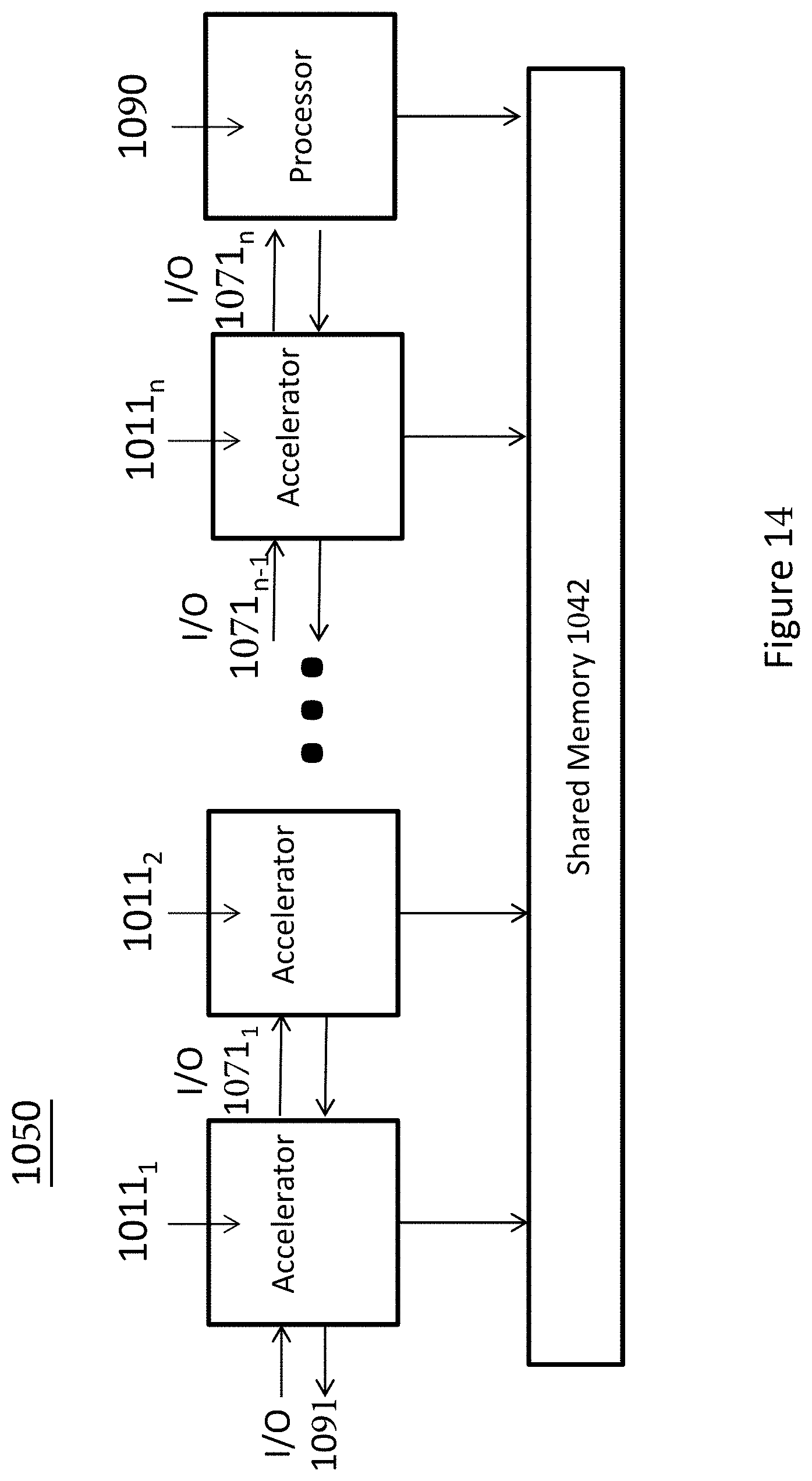
D00015

D00016

D00017

D00018

D00019
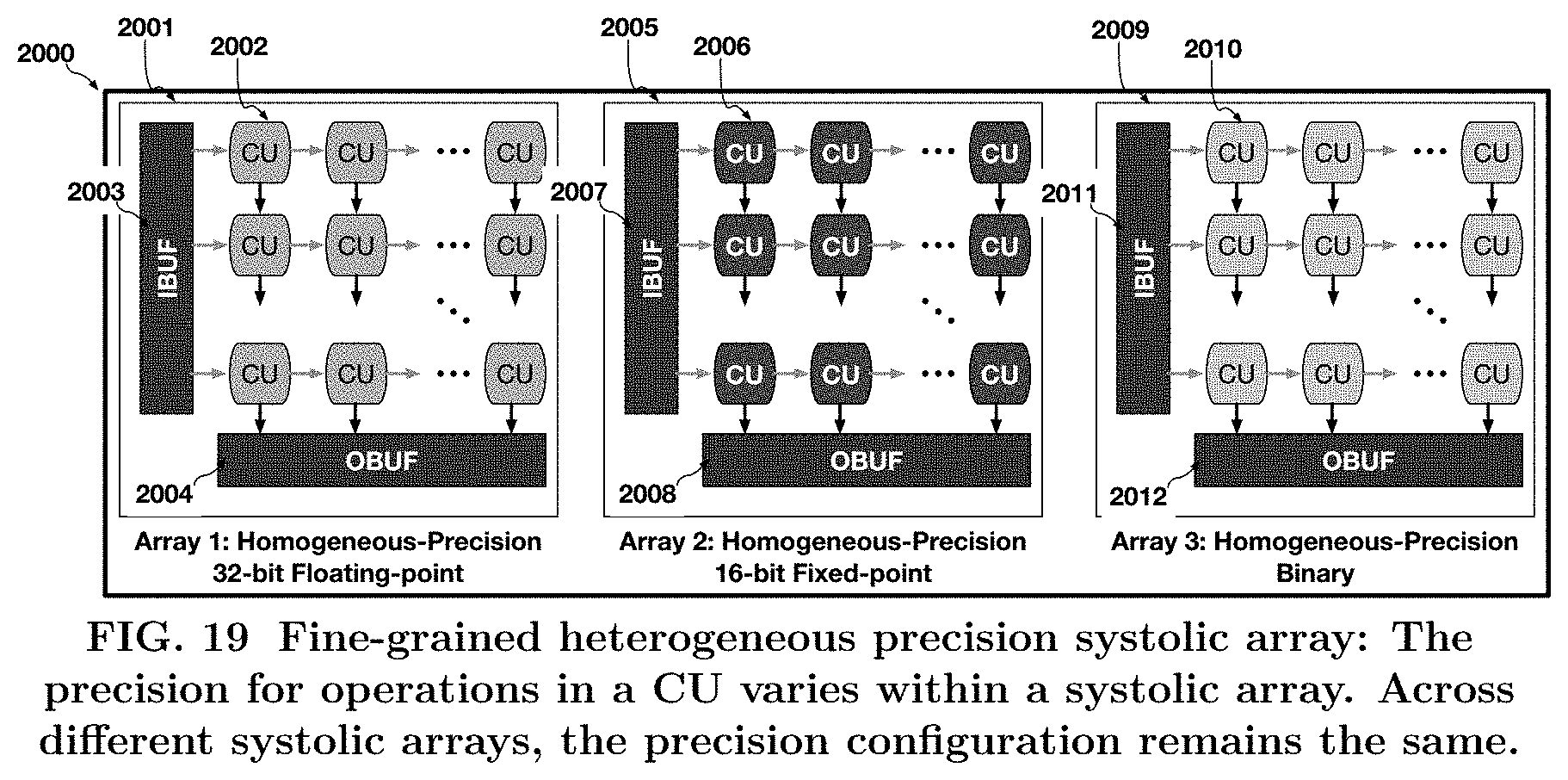
D00020
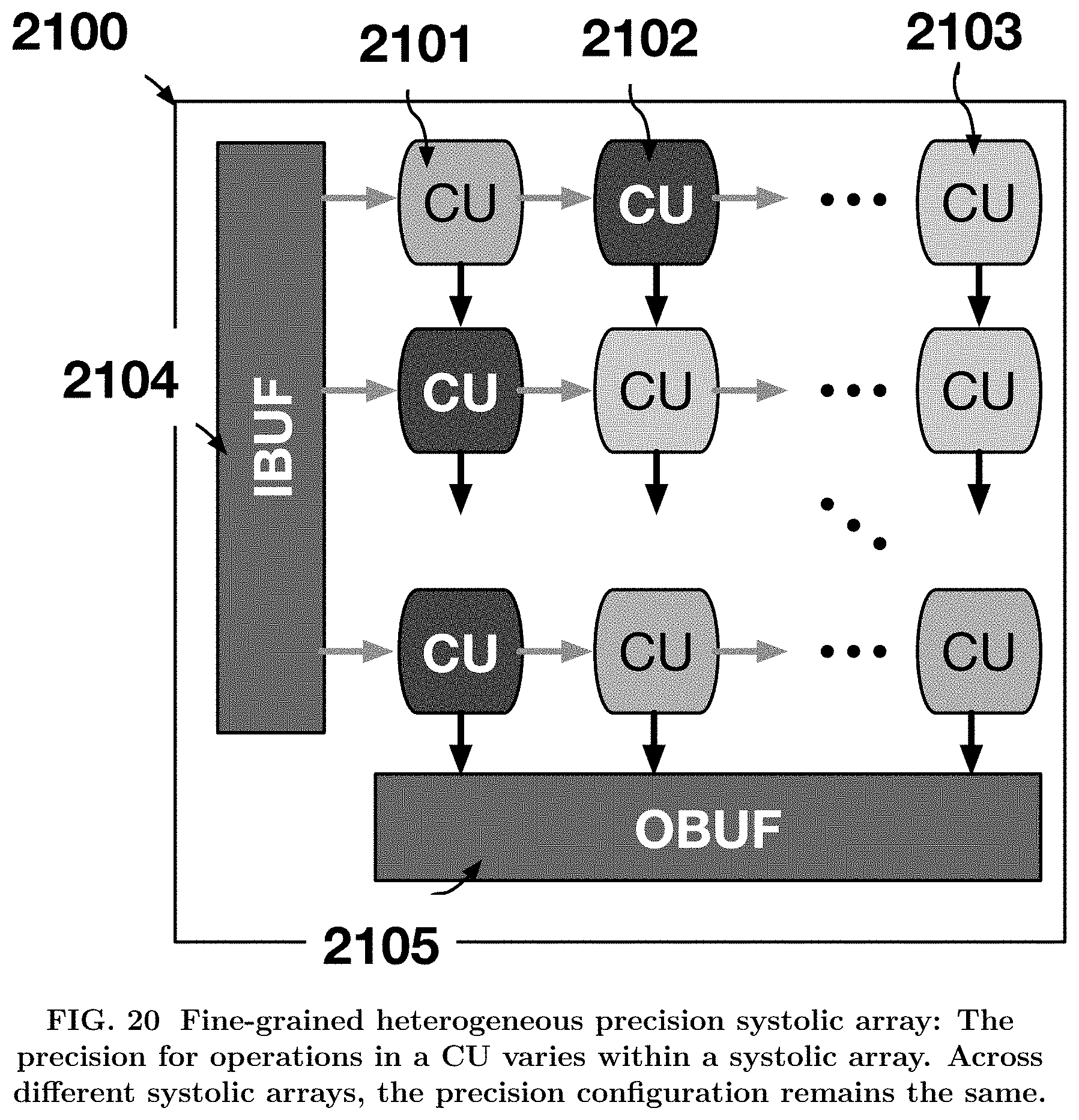
D00021
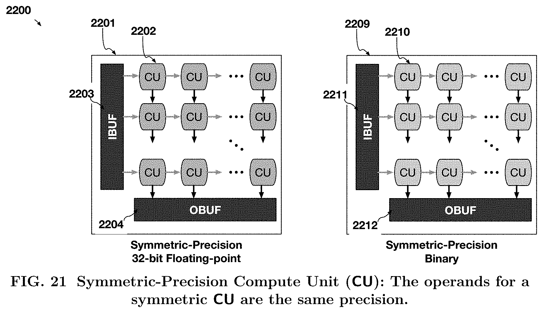
D00022

D00023

D00024

D00025

D00026

XML
uspto.report is an independent third-party trademark research tool that is not affiliated, endorsed, or sponsored by the United States Patent and Trademark Office (USPTO) or any other governmental organization. The information provided by uspto.report is based on publicly available data at the time of writing and is intended for informational purposes only.
While we strive to provide accurate and up-to-date information, we do not guarantee the accuracy, completeness, reliability, or suitability of the information displayed on this site. The use of this site is at your own risk. Any reliance you place on such information is therefore strictly at your own risk.
All official trademark data, including owner information, should be verified by visiting the official USPTO website at www.uspto.gov. This site is not intended to replace professional legal advice and should not be used as a substitute for consulting with a legal professional who is knowledgeable about trademark law.