Method And Arrangements For Hdr Encoding
STROM; Jacob ; et al.
U.S. patent application number 15/743235 was filed with the patent office on 2019-12-05 for method and arrangements for hdr encoding. This patent application is currently assigned to TELEFONAKTIEBOLAGET LM ERICSSON (PUBL). The applicant listed for this patent is TELEFONAKTIEBOLAGET LM ERICSSON (PUBL). Invention is credited to Kristofer DOVSTAM, Jacob STROM.
| Application Number | 20190373233 15/743235 |
| Document ID | / |
| Family ID | 57757454 |
| Filed Date | 2019-12-05 |


View All Diagrams
| United States Patent Application | 20190373233 |
| Kind Code | A1 |
| STROM; Jacob ; et al. | December 5, 2019 |
METHOD AND ARRANGEMENTS FOR HDR ENCODING
Abstract
A pixel in a picture is pre-processed by determining at least one bound for a luma component value of the pixel in a second color space based on a transfer function of a desired linear luminance value of the pixel in a third color space. A luma component value in the second color space is then selected for the pixel within an interval comprising multiple luma component values in the second color space and 5 bounded by the at least one bound. A color of the pixel is represented by the luma component value and two chroma component values in the second color space. The pre-processing enables selection of a suitable luma component value for the pixel in a computationally efficient way by limiting the number of luma component values that are available for the particular pixel.
| Inventors: | STROM; Jacob; (Stockholm, SE) ; DOVSTAM; Kristofer; (Hasselby, SE) | ||||||||||
| Applicant: |
|
||||||||||
|---|---|---|---|---|---|---|---|---|---|---|---|
| Assignee: | TELEFONAKTIEBOLAGET LM ERICSSON
(PUBL) Stockholm SE |
||||||||||
| Family ID: | 57757454 | ||||||||||
| Appl. No.: | 15/743235 | ||||||||||
| Filed: | June 14, 2016 | ||||||||||
| PCT Filed: | June 14, 2016 | ||||||||||
| PCT NO: | PCT/SE2016/050572 | ||||||||||
| 371 Date: | January 9, 2018 |
Related U.S. Patent Documents
| Application Number | Filing Date | Patent Number | ||
|---|---|---|---|---|
| 62190906 | Jul 10, 2015 | |||
| Current U.S. Class: | 1/1 |
| Current CPC Class: | H04N 9/77 20130101; H04N 5/20 20130101; H04N 9/68 20130101; H04N 19/85 20141101; H04N 19/182 20141101; H04N 19/186 20141101 |
| International Class: | H04N 9/68 20060101 H04N009/68; H04N 19/186 20060101 H04N019/186; H04N 19/182 20060101 H04N019/182 |
Claims
1. A method of pre-processing a pixel in a picture, said method comprising: determining at least one bound for a luma component value of said pixel in a second color space based on a function of a desired linear luminance value of said pixel in a third color space, wherein said function is a transfer function; and selecting a luma component value in said second color space for said pixel within an interval comprising multiple luma component values in said second color space and bounded by said at least one bound, wherein a color of said pixel is represented by said luma component value, a first chroma component value and a second chroma component value in said second color space.
2. The method of claim 1, further comprising determining said desired linear luminance value based on a linear color of said pixel in a first color space.
3. The method of claim 1, wherein determining said at least one bound comprises determining an upper bound for said luma component value and for said interval as tf(Y.sub.o), wherein tf( ) is a concave transfer function and Y.sub.o denotes said desired linear luminance value.
4-5. (canceled)
6. The method of claim 1, wherein determining said at least one bound comprises determining a lower bound for said luma component value and for said interval as tf(Y.sub.o), wherein tf( ) is a monotonously increasing transfer function and Y.sub.o denotes said desired linear luminance value.
7. (canceled)
8. The method of claim 1, wherein selecting said luma component value comprises selecting, within said interval, a luma component value that minimizes a difference between said desired linear luminance value and a linear luminance value in said third color space calculated based on said luma component value, said first chroma component value and said second chroma component value in said second color space.
9. The method of claim 1, wherein selecting said luma component value comprises performing a binary search to select said luma component value within said interval.
10. The method of claim 9, wherein performing said binary search comprises: performing, as long as an upper bound for said luma component value is larger than a lower bound for said luma component value plus one, the following steps: determining a luma component value in the middle of an interval bounded by said lower bound and said upper bound; calculating a linear luminance value in said third color space based on said determined luma component value, said first chroma component value and said second chroma component value in said second color space; and setting said lower bound equal to said determined luma component value if said calculated linear luminance value is smaller than said desired linear luminance value or otherwise setting said upper bound equal to said determined luma component value; and selecting said luma component value as said lower bound or said upper bound.
11. The method of claim 10, wherein selecting said luma component value comprises: calculating a first linear luminance value based on said lower bound and said first chroma component value and said second chroma component value in said second color space; calculating a first difference between said first linear luminance value, or a function of said first linear luminance value, and said desired linear luminance value, or said function of said desired linear luminance value; calculating a second linear luminance value based on said upper bound and said first chroma component value and said second chroma component value in said second color space; calculating a second difference between said second linear luminance value, or said function of said second linear luminance value, and said desired linear luminance value, or said function of said desired linear luminance value; and selecting said lower bound as said luma component value in said second color space if said first difference is smaller than said second difference and otherwise selecting said upper bound as said luma component value in said second color space.
12. (canceled)
13. A device for pre-processing a pixel in a picture, wherein said device is configured to determine at least one bound for a luma component value of said pixel in a second color space based on a function of a desired linear luminance value of said pixel in a third color space, wherein said function is a transfer function; and said device is configured to select a luma component value in said second color space for said pixel within an interval comprising multiple luma component values in said second color space and bounded by said at least one bound, wherein a color of said pixel is represented by said luma component value, a first chroma component value and a second chroma component value in said second color space.
14. The device of claim 13, said device is configured to determine said desired linear luminance value based on a linear color of said pixel in a first color space.
15. The device of claim 13, wherein said device is configured to determine an upper bound for said luma component value and for said interval as tf(Y.sub.o), wherein tf() is a concave transfer function and Y.sub.o denotes said desired linear luminance value.
16-17. (canceled)
18. The device of claim 13, wherein said device is configured to determine a lower bound for said luma component value and for said interval as tf(Y.sub.o), wherein tf() is a monotonously increasing transfer function and Y.sub.o denotes said desired linear luminance value.
19. (canceled)
20. The device of claim 13, wherein said device is configured to select, within said interval, a luma component value that minimizes a difference between said desired linear luminance value and a linear luminance value in said third color space calculated based on said luma component value, said first chroma component value and said second chroma component value in said second color space.
21. The device of claim 13, wherein said device is configured to perform a binary search to select said luma component value within said interval.
22. The device of claim 21, wherein said device is configured to perform, as long as an upper bound for said luma component value is larger than a lower bound for said luma component value plus one: determine a luma component value in the middle of an interval bounded by said lower bound and said upper bound; calculate a linear luminance value in said third color space based on said determined luma component value, said first chroma component value and said second chroma component value in said second color space; and set said lower bound equal to said determined luma component value if said calculated linear luminance value is smaller than said desired linear luminance value or otherwise set said upper bound equal to said determined luma component value; and said device is configured to select said luma component value as said lower bound or said upper bound.
23. The device of claim 22, wherein said device is configured to calculate a first linear luminance value based on said lower bound, said first chroma component value and said second chroma component value in said second color space; said device is configured to calculate a first difference between said first linear luminance value, or a function of said first linear luminance value, and said desired linear luminance value, or said function of said desired linear luminance value; said device is configured to calculate a second linear luminance value based on said upper bound, said first chroma component value and said second chroma component value in said second color space; said device is configured to calculate a second difference between said second linear luminance value, or said function of said second linear luminance value, and said desired linear luminance value, or said function of said desired linear luminance value; and said device is configured to select said lower bound as said luma component value in said second color space if said first difference is smaller than said second difference and otherwise selecting said upper bound as said luma component value in said second color space.
24. The device of claim 13, further comprising: a processor; and a memory comprising instructions executable by said processor, wherein said processor is operative to determine said at least one bound for said luma component value; and said processor is operative to select said luma component value in said second color space for said pixel within said interval.
25. (canceled)
26. A device for encoding a pixel in a picture, said device comprises: a processor; and a memory comprising instructions executable by said processor, wherein said processor is operative to determine at least one bound for a luma component value of said pixel in a second color space based on a function of a desired linear luminance value of said pixel in a third color space, wherein said function is a transfer function; said processor is operative to select a luma component value in said second color space for said pixel within an interval comprising multiple luma component values in said second color space and bounded by said at least one bound; and said processor is operative to encode said luma component value, a subsampled first chroma component value and a subsampled second chroma component value in said second color space.
27. (canceled)
28. A user equipment comprising a device of claim 13, wherein said user equipment is selected from a group consisting of a computer, a laptop, a smart phone, a tablet and a set-top box.
29. A computer program comprising instructions, which when executed by a processor, cause said processor to determine at least one bound for a luma component value of a pixel in a second color space based on a function of a desired linear luminance value of said pixel in a third color space, wherein said function is a transfer function; and select a luma component value in said second color space for said pixel within an interval comprising multiple luma component values in said second color space and bounded by said at least one bound, wherein a color of said pixel is represented by said luma component value, a first chroma component value and a second chroma component value in said second color space.
30-33. (canceled)
Description
TECHNICAL FIELD
[0001] The present embodiments generally relate to pre-processing and encoding of pixels in a picture, and in particular to such pre-processing and encoding that improves luminance values of pixels in a computational efficient way.
BACKGROUND
[0002] Within the art of video coding, a non-linear transfer function converts linear samples to non-linear samples with the purpose to mimic human vision. In coding of HDR (High Dynamic Range) video, it can be advantageous to use a highly non-linear transfer function, since this makes it possible to distribute many codewords to dark regions, and fewer codewords to bright regions, where the relative difference in brightness is anyway small.
[0003] Unfortunately, a combination of a highly non-linear transfer function, 4:2:0 subsampling and non-constant luminance ordering gives rise to severe artifacts in saturated colors, if traditional processing is used.
[0004] A simple example of a non-linear transfer function is x.sup.(1/gamma), wherein gamma is 2.2. One example of another transfer function is the one used in SMPTE specification ST 2084 [1]. Before display the inverse of the non-linear transfer function is used. In the gamma example, x.sup.(gamma) is used to go back to linear samples.
[0005] One example of traditional processing is the way to carry out conversion from RGB 4:4:4 to Y'CbCr 4:2:0 that is described in [2], which we will refer to as the "anchor" way of processing in this document. In this case RGB 4:4:4 is transferred by a non-linear transfer function to R'G'B' 4:4:4, which then is converted to Y'CbCr 4:4:4 by a linear color transform. Finally, the chroma samples Cb and Cr are subsampled to quarter resolution resulting in Y'CbCr 4:2:0. As described in the input contribution M35841 [3] to MPEG, the anchor way of processing gives rise to situations where changes between two colors of similar luminance can result in a reconstructed image with very different luminances.
SUMMARY
[0006] It is a general objective to provide an efficient pre-processing and encoding of pixels in a picture that improves luminance values of the pixels.
[0007] This and other objectives are met by embodiments as described herein.
[0008] An aspect of the embodiments relates to a method of pre-processing a pixel in a picture. The method comprises determining at least one bound for a luma component value of the pixel in a second color space based on a function of a desired linear luminance value of the pixel in a third color space. The function is preferably a transfer function. The method also comprises selecting a luma component value in the second color space for the pixel within an interval comprising multiple luma component values in the second color space and bounded by the at least one bound. A color of the pixel is then represented by the luma component value, a first chroma component value and a second chroma component value in the second color space.
[0009] Another aspect of the embodiments relates to a device for pre-processing a pixel in a picture. The device is configured to determine at least one bound for a luma component value of the pixel in a second color space based on a function of a desired linear luminance value of the pixel in a third color space, wherein the function is a transfer function. The device is also configured to select a luma component value in the second color space for the pixel within an interval comprising multiple luma component values in the second color space and bounded by the at least one bound, wherein a color of the pixel is represented by the luma component value, a first chroma component value and a second chroma component value in the second color space.
[0010] A further aspect of the embodiments relates to a device for pre-processing a pixel in a picture. The device comprises a determining unit for determining at least one bound for a luma component value of the pixel in a second color space based on a function of a desired linear luminance value of the pixel in a third color space. The function is a transfer function. The device also comprises a selector for selecting a luma component value in the second color space for the pixel within an interval comprising multiple luma component value sin the second color space and bounded by the at least one bound.
[0011] Another aspect of the embodiments relates to a device for encoding a pixel in a picture. The device comprises a processor and a memory comprising instructions executable by the processor. The processor is operative to determine at least one bound for a luma component value of the pixel in a second color space based on a function of a desired linear luminance value of the pixel in a third color space. The function is a transfer function. The processor is also operative to select a luma component value in the second color space for the pixel within an interval comprising multiple luma component value sin the second color space and bounded by the at least one bound. The processor is further operative to encode the luma component value, a subsampled first chroma component value and a subsampled second chroma component value in the second color space.
[0012] Yet another aspect of the embodiments relates to a device for encoding a pixel in a picture. The device comprises a determining unit for determining at least one bound for a luma component value of the pixel in a second color space based on a function of a desired linear luminance value of the pixel in a third color space. The function is a transfer function. The device also comprises a selector for selecting a luma component value in the second color space for the pixel within an interval comprising multiple luma component values in the second color space and bounded by the at least one bound. The device further comprises an encoder for encoding the luma component value, a subsampled first chroma component value and a subsampled second chroma component value in the second color space.
[0013] A further aspect of the embodiments relates to a computer program comprising instructions, which when executed by a processor, cause the processor to determine at least one bound for a luma component value of the pixel in a second color space based on a function of a desired linear luminance value of the pixel in a third color space. The function is a transfer function. The processor is also caused to select a luma component value in the second color space for the pixel within an interval comprising multiple luma component value sin the second color space and bounded by the at least one bound.
[0014] A related aspect of the embodiments defines a carrier comprising a computer program according to above. The carrier is one of an electric signal, an optical signal, an electromagnetic signal, a magnetic signal, an electric signal, a radio signal, a microwave signal, or a computer-readable storage medium.
[0015] An additional aspect of the embodiments relates to a signal representing an encoded version of a pixel in a picture. The encoded version comprises an encoded version of two subsampled chroma component values in a second color format and an encoded version of a luma component value in the second color format obtained according to any of the embodiments.
[0016] The pre-processing enables selection of a suitable luma component value for the pixel in a computationally efficient way by limiting the number of luma component values that are available for the particular pixel. This implies that the quality of the pixel as assessed by the luminance value for the pixel can be improved in a computationally efficient way.
BRIEF DESCRIPTION OF THE DRAWINGS
[0017] The embodiments, together with further objects and advantages thereof, may best be understood by making reference to the following description taken together with the accompanying drawings, in which:
[0018] FIG. 1 is a flow chart illustrating a method of pre-processing a pixel in a picture according to an embodiment;
[0019] FIG. 2 is a flow chart illustrating an additional, optional step of the method shown in FIG. 1 according to an embodiment;
[0020] FIG. 3 is a diagram plotting the convex function tf.sup.-1(x);
[0021] FIG. 4 is a flow chart illustrating an embodiment of the determining step in FIG. 1;
[0022] FIG. 5 is a flow chart illustrating an embodiment of the selecting step in FIG. 1;
[0023] FIG. 6 is a flow chart illustrating an embodiment of the selecting step in FIG. 5;
[0024] FIG. 7 is a flow chart illustrating an additional step of the method shown in FIG. 1 to form a method of encoding a pixel according to an embodiment;
[0025] FIG. 8 is a schematic illustration of hardware implementations of a device according to the embodiments;
[0026] FIG. 9 is a schematic illustration of an implementation of a device according to the embodiments with a processor and a memory;
[0027] FIG. 10 is a schematic illustration of a user equipment according to an embodiment;
[0028] FIG. 11 is a schematic illustration of an implementation of a device according to the embodiments with function modules;
[0029] FIG. 12 schematically illustrate a distributed implementation of the embodiments among multiple network devices;
[0030] FIG. 13 is a schematic illustration of an example of a wireless communication system with one or more cloud-based network devices according to an embodiment;
[0031] FIG. 14 illustrates an embodiment of deriving the corrected Y';
[0032] FIG. 15 is a diagram illustrating that there can be different linearizations in different color areas;
[0033] FIG. 16 illustrates Barten's curve for contrast sensitivity;
[0034] FIG. 17 illustrates a comparison between Rec709 and BT.2020 color gamuts;
[0035] FIG. 18 illustrates an embodiment of obtaining Cb' and Cr' by subsampling in linear RGB and obtaining Y' by using Ajusty;
[0036] FIG. 19 illustrates an embodiment of creating references with chroma upsampling in a representation invariant to intensity;
[0037] FIG. 20 illustrates an embodiment of iterative refinement of Cb' and Cr';
[0038] FIGS. 21A and 21B schematically illustrate performing the Ajusty processing chain in sequential passes;
[0039] FIG. 22A illustrate differences between deriving luma component values according to the anchor processing chain and the Ajusty processing chain; and
[0040] FIG. 22B schematically illustrate the quotient of maxRGB/(minRGB+s) for the picture shown in FIG. 22A.
DETAILED DESCRIPTION
[0041] Throughout the drawings, the same reference numbers are used for similar or corresponding elements.
[0042] The present embodiments generally relate to pre-processing and encoding of pixels in a picture, and in particular to such pre-processing and encoding that improves luminance values of pixels in a computationally efficient way.
[0043] A traditional compression chain involves the anchor way of pre-processing pictures of a video sequence. This pre-processing comprises feeding pixels of incoming linear red, green blue (RGB) light, typically ranging from 0 to 10,000 cd/m.sup.2, to an inverse transfer function, which results in new pixel values between 0 and 1. After this, the pixels undergo color transform resulting in a luma component (Y') and two chroma components (Cb, Cr). Then, the two chroma components are subsampled, such as to 4:2:0 or 4:2:2. The luma and subsampled chroma components are then encoded, also referred to as compressed herein. After decoding, also referred to as decompression herein, the 4:2:0 or 4:2:2 sequences are upsampled to 4:4:4, inverse color transformed and finally a transfer function gives back pixels of linear RGB light that can be output on a monitor for display.
[0044] A combination of a highly non-linear transfer function, chroma subsampling and non-constant luminance ordering gives rise to severe artifacts to the video data, in particular for saturated colors.
[0045] The pre-processing of pixels according to the embodiments can be used to combat or at least reduce the impact of artifacts, thereby resulting in a color that is closer to the incoming "true" color of a pixel.
[0046] A color space or color domain is the type and number of colors that originate from the combinations of color components of a color model. A color model is an abstract configuration describing the way colors can be represented as tuples of numbers, i.e. color components. The color components have several distinguishing features such as the component type, e.g. hue, and its unit, e.g. degrees or percentage, or the type of scale, e.g. linear or non-inear, and its intended number of values referred to as the color depth or bit depth.
[0047] Non-limiting, but illustrative, color spaces that are commonly used for pixels in pictures and videos include the red, green, blue (RGB) color space, the luma, chroma blue and chroma red (Y'CbCr, sometimes denoted Y'CbCr, Y'Cb'Cr', YC.sub.BC.sub.R, Y'C.sub.BC.sub.R Y'C.sub.B'C.sub.R' or YUV, Y.sub.UV, or D'.sub.YD'.sub.CBD'.sub.CR or E'.sub.YE'.sub.CBE'.sub.CR) color space and the luminance and chrominances (XYZ) color space.
[0048] In this document, the following terminology will be used.
[0049] RGB: Linear RGB values, where each value is proportional to the cd/m.sup.2 ("number of photons").
[0050] XYZ: Linear XYZ values, where each value is a linear combination of RGB. Y is called "luminance" and loosely speaking reflects well what the eye perceives as `brightness`.
[0051] R`G`B': Non-linear RGB values. R'=pq(R), G'=pq(G), B'=pq(B), pq() being a non-linear function. An example of a non-linear function is the Perceptual Quantizer (PQ) transfer function.
[0052] Y'CbCr A non-linear representation where each value is a linear combination of R', G' and B'. Y' is called "luma", and Cb and Cr are collectively called "chroma". This is to distinguish Y' from luminance, since Y also contains some chrominance, and Cb and Cr also contain some luminance.
[0053] ICtCp: A representation of color designed for HDR and Wide Color Gamut (WCG) imagery and is intended as an alternative to Y'Cb'Cr'. I represents intensity and is a representation of luma information, whereas CtCp carries chroma information.
[0054] FIG. 1 is a flow chart illustrating a method of pre-processing a pixel in a picture. The method comprises determining, in step S1, at least one bound for a luma component value of the pixel in a second color space based on a function of a desired linear luminance value of the pixel in a third color space. The function is preferably a transfer function. The method then continues to step S2, which comprises selecting a luma component value in the second color space for the pixel within an interval comprising multiple luma component values in the second color space and bounded by the at least one bound. A color of the pixel is then represented by the luma component value as selected in step S2, a first chroma component value and a second chroma component value in the second color space.
[0055] The method of pre-processing comprising step S1 and S2 is performed on at least one pixel in a picture comprising multiple pixels. The method could be advantageously be applied to multiple, i.e. at least two, pixels in the picture, such as all pixels within a region of the picture or indeed all pixels in the picture, which is schematically illustrated by the line L1 in FIG. 1. The picture is preferably a picture of a video sequence comprising a plurality of pictures, such as a HDR or WCG video sequence. In such a case, the method could be applied to pixels in multiple different pictures of the video sequence. For instance, the method could be applied to all pictures in the video sequence, or to selected pictures within the video sequence. Such selected pictures could, for instance be, so called random access point (RAP) or intra RAP (IRAP) pictures and/or pictures belonging to a lowest layer in a multi-layer video sequence or a base layer in a multi view video sequence.
[0056] Step S1 of FIG. 1 thereby determines at least one bound for the luma component value in the second color space. This at least one bound is, in an embodiment, an upper bound for the luma component value. In this embodiment, the upper bound corresponds to the largest value for the luma component value in the second color space, i.e. luma component value .ltoreq.upper bound.
[0057] In another embodiment, the at least one bound determined in step S1 is a lower bound for the luma component value in the second color space. In this embodiment, the lower bound thereby corresponds to the smallest value for the luma component value in the second color space, i.e. luma component value 2 lower bound.
[0058] It is also possible, in an embodiment, to determine both a lower bound and an upper bound for the luma component value in the second color space in step S1, i.e. lower bound .ltoreq.luma component value .ltoreq.upper bound.
[0059] The at least one bound, i.e. lower and/or upper bound, is determined in step S1 based on a transfer function of a desired linear luminance value of the pixel in a third color space, i.e. a color space different from the second color space.
[0060] In a particular embodiment, the luma component value in the second color space is a Y'value in the Y'CbCr color space. The first and second chroma component values are, in this particular embodiment, Cb and Cr values. In this particular embodiment, the linear luminance value in the third color space is a Y value in the XYZ color space. Herein, the subscript "o" is used to denote the "original" or desired luminance value in the third color space, e.g. Y.sub.o value in XYZ color space. In such a case, the upper bound Y'.sub.highest=f.sub.1(tf.sub.1(Y.sub.o)) and/or the lowest bound Y'.sub.lowest=f.sub.2(tf.sub.2(Y.sub.o)), wherein tf.sub.1() and tf.sub.2() denote respective transfer functions and f.sub.1() and f.sub.2( ) denote respective functions. Note that the inverse tf.sup.-1() of a transfer function tf() is also a transfer function.
[0061] The at least one bound determined in step S1 encloses or bounds an interval comprising multiple luma component values in the second color space. In the case of determining an upper bound in step S1, the interval is thereby bounded in its upper end, i.e..ltoreq.Y'.sub.highest. The luma component in the second color space can, in an embodiment, only assume values equal to or larger than a minimum value or, for instance 0 or 64. Hence, in such an embodiment, the interval is defined as [0, Y'.sub.highest] or [64, Y'.sub.highest].
[0062] Correspondingly, if step S1 comprises determining a lower bound, the interval is thereby bounded in its lower end, i.e..gtoreq.Y'.sub.lowest. In an embodiment, a luma component value cannot assume a value higher than a maximum value of, for instance, 1.0, 940 or 2.sup.N-1, wherein N represents the number of bits available for representing the luma component value. For instance, in the case of HDR video N is preferably 10, i.e. resulting in 2.sup.10-1=1023. Hence, in such an embodiment, the interval is defined as [Y'.sub.lowest, 1.0], [Y'.sub.lowest, 940] or [Y'.sub.lowest, 2.sup.N-1], such as for instance [Y'.sub.lowest, 1023].
[0063] If both the upper and lower bounds are determined in step S1, then the interval is defined as [Y'.sub.lowest, Y'.sub.highest].
[0064] It is possible that the calculated value Y'.sub.highest will be higher than the maximum value, for instance 1.0, 940 or 2.sup.N-1, such as 1023. In such a case, the upper bound determined in step S1 is preferably determined to be equal to the maximum value. Correspondingly, it is possible that the calculated value Y'.sub.lowest will be lower than the minimum value, for instance 0 or 64. In such a case, the lower bound determined in step S1 is preferably determined to be equal to the minimum value.
[0065] Unless Y'.sub.highest is equal to or larger than the maximum value and Y'.sub.lowest is equal to or lower than the minimum value, the interval bounded by the at least one bound determined in step S1 constitutes a sub-interval of the allowed range of values for the luma component in the second color space, i.e. a sub-interval of [minimum value, maximum value], for instance a sub-interval of [0.0, 1.0], [64, 940] or [0, 1023].
[0066] The interval [64, 940] is generally used for representing the luma component value Y' in HDR video as above but it may also be possible to use the interval [0, 1023]. The corresponding interval for standard range video (SDR) is [64, 940] for the luma component value Y'. Thus, in an embodiment directed toward SDR video the interval bounded by the at least one bound determined in step S1 constitutes a sub-interval of the allowed range of value for the luma component in the second color space, i.e. a sub-interval of [64, 940].
[0067] This means that the interval from which a luma component value in the second color space is selected for the pixel in step S2 only constitutes a portion of all allowable luma component values. This means that the at least one bound determined in step S1 limits the value the luma component can assume for the current pixel since the luma component value can only be selected from within the interval instead of within the whole allowable range of [minimum value, maximum value].
[0068] FIG. 2 is a flow chart illustrating an additional optional step of the method shown in FIG. 1. The method starts in step S10, which comprises determining the desired linear luminance value based on a linear color of the pixel in a first color space. The method then continues to step S1 in FIG. 1, where the determined desired linear luminance is used to determine the at least one bound.
[0069] This linear color of the pixel in the first color space is preferably the color of the pixel as input to the pre-processing. In a particular embodiment, this linear color is an RGB color in the RGB color space. This linear color is sometimes denoted R.sub.oG.sub.oB.sub.o herein to indicate that it represent the original color of the pixel.
[0070] The desired linear luminance value in the third color space can then be determined by application of a color transform to the linear color in the first color space, preferably an RGB-to-XYZ color transform, such as the color transform in equation 1 when RGB originates from BT.2020 or equation 2 when RGB originates from BT.709, also referred to as Rec709:
X=0.636958R+0.144617G+0.168881B
Y=0.262700R+0.677998G+0.059302B
Z=0.000000R+0.028073G+1.060985B (equation 1)
X=0.412391R+0.357584G+0.180481B
Y=0.212639R+0.715169G+0.072192B
Z=0.019331R+0.119195G+0.950532B (equation 2)
[0071] In fact, only the second line in equation 1 or 2 need to be calculated to obtain the desired linear luminance value (Y.sub.o) from the linear color (R.sub.oG.sub.oB.sub.o) in the first color space; Y.sub.o=0.262700R.sub.o+0.677998G.sub.o+0.059302B.sub.o or Y.sub.o=0.212639R.sub.o+0.715169G.sub.o+0.072192B.sub.0.
[0072] In a first embodiment, step S1 of FIG. 1 comprises determining an upper bound for the luma component value and thereby for the interval based on, preferably as, tf(Y.sub.o). In this embodiment tf() is a concave transfer function and Y.sub.o denotes the desired linear luminance value.
[0073] The transfer function tf() is in this embodiment a concave transfer function, which means that the inverse of the transfer function tf.sup.-1() is a convex transfer function. The defining characteristic of a convex function f() is the property that if x.sub.1 and x.sub.2 are two different values, and t is a value in the interval [0, 1], then f(tx.sub.1+(1-t)x.sub.2).ltoreq.tf(x.sub.1)+(1-t)f(x.sub.2).
[0074] The concave transfer function can be any concave transfer function defined on the interval [0, 1]. A particular example of such a concave transfer function is the gamma function y=x.sup.(1/gamma), wherein gamma is, for instance, 2.2.
[0075] Here below a particular implementation example of determining the upper bound Y'es according to the first embodiment is described in more detail. In this implementation example, luma and chroma component values in the second color space are exemplified as Y' and CbCr values, respectively, in the Y'CbCr color space. Correspondingly, the linear luminance value in the third color space is exemplified as a Y value in the XYZ color space.
[0076] In order to see how Y'.sub.highest can be calculated, we first study how the linear luminance Y is calculated from a combination of Y'CbCr quantied to 10 bits, i.e. Y'10 bit, Cb10bit and Cr10bit.
[0077] 1. First convert from Y'10 bit, Cb10bit and Cr10 bit to values Y' in the interval [0, 1] and Cb, Cr in the interval [-0.5, 0.5]:
Y'=(Y'10 bit/4.0-16.0)/219.0
Cb=dClip((Cb10bit/4.0-128.0)/224.0, -0.5,0.5)
Cr=dCip((Cr10bit/4.0-128.0)/224.0, -0.5,0.5)
[0078] The clipping function dClip(x, a, b) clips the value x to the interval [a, b], i.e. outputs a if x<a, outputs b if x>b and otherwise outputs x.
[0079] 2. The Y', Cb, Cr values are then converted into R'G'B' using a color transform, such as defined in equation 3:
R'=Y'+a.sub.12*Cb+a.sub.13'Cr
G'=Y+a.sub.22Cb+a.sub.23*Cr
B'=Y'+a.sub.32Cb+a.sub.33Cr (equation 3)
[0080] In equation 3, the constants a.sub.12=0 and a.sub.33=0, whereas the other constant values depend on the color space. Thus, for color space Rec.709 we have a.sub.13=1.57480, a.sub.2=-0.18733, a.sub.23=-0.46813, a.sub.32=1.85563 and for BT.2020 we have a.sub.13=1.47460, a.sub.22=-0.16455, a.sub.23=-0.57135, a.sub.32=1.88140.
[0081] The non-linear color R'G'B' is then dipped within the interval [0, 1]:
R'.sub.01=dClip(R',0,1)
G'.sub.01=dClip(G',0,1)
B'.sub.01=dClip(B',0,1)
[0082] The subscript 01 is to mark that the values have been dipped to the interval [0,1].
[0083] 3. The non-linear color R'G'B' is then converted to linear light RGB by applying the electro-optical transfer function EOTF, which is defined in equation C1 in Annex C.
R=tf.sup.-1(R'.sub.01)
G=tf.sup.-1(G'.sub.01)
B=tf.sup.-1(B'.sub.01)
[0084] 4. Finally the resulting linear luminance value or light Y.sub.result is calculated from from the RGB using
Y.sub.result=w.sub.R*R+w.sub.G*G+w.sub.B*B,
[0085] where w.sub.R=0.212639, w.sub.G=0.715169, w.sub.B=0.072192 for Rec.709 and where w.sub.R=0.262700, w.sub.G=0.677998, w.sub.B=0.059302 for BT.2020.
[0086] The resulting linear luminance Y.sub.result that is obtained by following steps 1 through 4 above can, thus, be written as a function of R'.sub.01, G'.sub.01 and B'.sub.01:
Y.sub.result=w.sub.RR+w.sub.GG+w.sub.BB=w.sub.Rtf.sup.-1(R'.sub.01)+w.su- b.Gtf.sup.-1(G'.sub.01)+w.sub.Btf.sup.-1(B'.sub.01) (equation 4)
[0087] Now comes a crucial observation. The transfer function tf() is, in this embodiment, concave, which means that the inverse tf.sup.-1() is convex. This can easily be seen by plotting tf.sup.-1(x) for the valid range of x from [0, 1], as is done in FIG. 3. The defining characteristic of a convex function f() is the property that if x.sub.1 and x.sub.2 are two values, and t is a value in the interval [0, 1], then f(t.sub.x+(1-t)x.sub.2).ltoreq.tf(x.sub.1)+(1-t)f(x.sub.2). This can be generalized to three values, see Annex A. Assume x.sub.1, x.sub.2 and x.sub.3 are three values, and that we have three values w.sub.1, w.sub.2 and w.sub.3 such that w.sub.1+w.sub.2+w.sub.3=1. If f() is convex the following inequality holds f(w.sub.1x.sub.1+w.sub.2x.sub.2+w.sub.3x.sub.3).ltoreq.w.sub.1f(x.sub.1)+- w.sub.2f(x.sub.2)+w.sub.3f(x.sub.3).
[0088] We will prove this statement in Annex A, but for now we just assume it holds. We can use this on the value for Y from equation 4. Since tf-1(x) is convex, we get
Y.sub.result=w.sub.Rtf.sup.-1(R'.sub.01)+w.sub.Gtf.sup.-1(G'.sub.01)+w.s- ub.Btf.sup.-1(B'.sub.01).gtoreq.tf.sup.-1(w.sub.RR'.sub.01+w.sub.GG'.sub.0- 1+w.sub.BB'.sub.01) (equation 5)
[0089] Inserting the values for R', G' and B' from step 2 above and ignoring for a while the clipping, i.e. assuming that R'.sub.01=R', and the same applies to the G and B color components, we get
Y.sub.result.gtoreq.tf.sup.-1(w.sub.RR'+w.sub.GG'+w.sub.BB') (equation 6)
[0090] Now we can compare this with the definition of Y' for BT.2020 in 2.4.6.3 in [4], replicated here for the convenience of the reader, Y'=0.2627R'+0.6780G'+0.0593B'.
[0091] Remember that for BT.2020, w.sub.R=0.262700, w.sub.G=0.677998, w.sub.B=0.059302. This is no coincidence, the Y'CbCr color conversion uses the same coefficients to calculate Y' as is used to calculate Y in XYZ. This means that, modulo rounding errors which do not matter, the expression w.sub.RR'+w.sub.GG'+w.sub.BB' is equal to Y'. We can therefore conclude that Y.sub.result.gtoreq.tf.sup.-1(Y'), and by applying the transfer function tf() on both sides, we get that Y'.ltoreq.tf(Y.sub.result).
[0092] We can therefore say, that if we want a certain result Y.sub.result, our Y' must be smaller than tf(Y.sub.result). In particular, if we want the result to be the desired linear luminance Y.sub.o, we must make sure that Y' is smaller than tf(Y.sub.o). Hence we have Y'.ltoreq.tf(Y.sub.o)=Y'.sub.highest.
[0093] We have therefore come up with an upper bound on Y', i.e. a highest value that Y' can take, namely Y'.sub.highest, and we also have a convenient way of calculating it--just compute the desired linear luminance Y.sub.o of the pixel and feed it through the transfer function.
[0094] In a second embodiment, step S1 of FIG. 1 comprises determining an upper bound for the luma component value and for the interval as a maximum of tf(Y.sub.o)-a.sub.13Cr, tf(Y.sub.o)-a.sub.22Cb-a.sub.23Cr and tf(Y.sub.o)-a.sub.32Cb. In this embodiment, the transfer function tf() is a monotonously increasing transfer function, Y.sub.o denotes the desired linear luminance value, Cb denotes the first chroma component value in the second color space, and Cr denotes the second chroma component value in the second color space. The constants a.sub.13=1.57480, a.sub.22=-0.18733, a.sub.23=-0.46813 and a.sub.32=1.85563 for Rec.709 and a.sub.13=1.47460, a.sub.22=-0.16455, a.sub.23=-0.57135 and a.sub.32=1.88140 for BT.2020.
[0095] Hence, in this embodiment the upper bound is equal to max(tf(Y.sub.o)-a.sub.13Cr, tf(Y.sub.o)-a.sub.22Cb-a.sub.23Cr, tf(Y.sub.o)-a.sub.32Cb), wherein max(a, b, c) outputs the largest of a, b and c.
[0096] Here below another particular implementation example of determining the upper bound Y'.sub.highest according to the second embodiment is described in more detail. In this implementation example, luma and chroma component values in the second color space are exemplified as Y' and CbCr values, respectively, in the Y'CbCr color space. Correspondingly, the linear luminance value in the third color space is exemplified as a Y value in the XYZ color space.
[0097] If we follow steps 1 through 4 described in the foregoing, equation 4 states that we get a resulting linear luminance or light value Y.sub.result according to
Y.sub.result=w.sub.RR+w.sub.GG+w.sub.BB=w.sub.Rtf.sup.-1(R'.sub.01)+w.su- b.Gtf.sup.-1(G'.sub.01)+w.sub.Btf.sup.-1(B'.sub.01) (equation 4)
[0098] Now we set M'.sub.01=min(R'.sub.01, G'.sub.01, B'.sub.01). Since the transfer function tf.sup.-1() is monotonically increasing this means that tf.sup.-1(M'.sub.01)=min(tf.sup.-1(R'.sub.01), tf.sup.-1(G'.sub.01), tf.sup.-1(B'.sub.01)). We can then write Y.sub.result.gtoreq.w.sub.Rtf.sup.-1(M'.sub.01)+w.sub.Gtf.sup.-1(M'.sub.0- 1)+w.sub.Btf.sup.-1(M'.sub.01), which can be simplified to Y.sub.result.gtoreq.(w.sub.R+w.sub.G+w.sub.B)tf.sup.-1(M'.sub.01), and, since (w.sub.R+w.sub.G+w.sub.B)=1, to Y.sub.result.gtoreq.tf.sup.-1(min(R'.sub.01, G'.sub.01, B'.sub.01)).
[0099] Now, we want to replace R'.sub.01, G'.sub.01, B'.sub.01 with the non-clipped variables R', G', B'. We do so in two steps, by first replacing R'.sub.01, G'.sub.01, B'.sub.01 with R'.sub.1, G'.sub.1, B'.sub.1 and then replacing R'.sub.1, G'.sub.1, B'.sub.1 with R', G', B' according to the following explanation. Let us assume the clipping is done according to the following steps, in which equation 3a corresponds to equation 3 but where the terms equal to zero due to a.sub.12=0 and a.sub.33=0 have been omitted:
R'=Y'+a.sub.13*Cr
G'=Y'+a.sub.22*Cb+a.sub.23*Cr
B'=Y'+a.sub.32*Cb
R'.sub.1=min(R',1)
G'.sub.1=min(G',1)
B'.sub.1=min(B',1)
R'.sub.01=max(R'.sub.1,0)
G'.sub.01=max(G'.sub.1,0)
B'.sub.01=max(B'.sub.1,0) (equation 3a)
[0100] Here R'.sub.1 is the value after we have clipped against 1, but before we have clipped against 0. This means that R'.sub.1.ltoreq.R'.sub.01, since if R'.sub.1 is larger than 0 they are the same, and if R'.sub.1 is smaller than 0, it is smaller. By analogous reasoning, G'.sub.1.ltoreq.G'.sub.o and B'.sub.1.ltoreq.B'.sub.01, which means that min(R'.sub.1, G'.sub.1, B'.sub.1).ltoreq.min(R'.sub.01, G'.sub.01, B'.sub.01) and, thus, Y.sub.result.gtoreq.tf.sup.-1(min(R'.sub.01, G'.sub.01, B'.sub.01)).gtoreq.tf.sup.-1(min(R'.sub.1, G'.sub.1, B'.sub.1)).
[0101] The next step is to replace R'.sub.1, G'.sub.1, B'.sub.1 with the non-clipped variables R', G', B'. We now make a crucial observation, namely that there exists no combination of Y', Cr and Cb so that all three variables R', G' and B' are simultaneously larger than 1. To see this, notice the signs of the variables a.sub.13, a.sub.22, a.sub.23 and a.sub.32: a.sub.13 and a.sub.32 are positive, and both a.sub.22 and a.sub.23 are negative. We can therefore write equation 3a as
R'=Y'+|a.sub.13|*Cr
G'=Y'-|a.sub.22|*Cb-|a.sub.23|*Cr
B'=Y'+|a.sub.32|*Cb
where |a| denotes the absolute value of a. Multiply each equation with -1,
R'=-Y'-|a.sub.13|*Cr
G'=-Y'+|a.sub.22|*Cb+|a.sub.23|*Cr
B'=-Y'-|a.sub.32|*Cb
[0102] Add 1 to each side of each equation,
1-R'=1-Y'-|a.sub.13|*Cr
1-G'=1-Y'+|a.sub.22|*Cb+|a.sub.23|*Cr
1-B'=1-Y'-|a.sub.32|*Cb
[0103] Now write this equation as,
R''=1-Y'-|a.sub.13|*Cr
G''=1-Y'+|a.sub.22|*Cb+|a.sub.23|*Cr
B''=1-Y'-|a.sub.32|*Cb
where R''=1-R', G''=1-G' and B''=1-B'. Showing that there exists no combination of Y', Cr and Cb so that all three variables R', G' and B' are simultaneously larger than 1, is the same as showing that there exists no combination of Y', Cr and Cb so that all three variables R'', G'' and B'' are simultaneously smaller than 0. Since Y' lies within the range [0, 1], we know that 1-Y' is never smaller than 0. Examining the signs of Cr and Cb, we see that If Cb>0 and Cr>0, then G''>0 If Cb>0 and Cr<0, then R''>0 If Cb<0 and Cr>0, then B''>0 If Cb<0 and Cr<0, then R'' and B''>0
[0104] Hence at least one of R'', G'', B'' must be positive, and hence at least one of R', G', B' is smaller than 1. This further means that the minimum, min(R', G', B'), is guaranteed to be smaller than 1. In particular, if min(R', G', B')=R', we know that R'<1 and hence R'=R'.sub.1. The same goes for G' and B', if they are the minimum of R', G' and B' they must equal their clipped version G'.sub.1 and B'.sub.1. Hence, we know that min(R', G', B')=min(R'.sub.1, G'.sub.1, B'.sub.1) and we can write Y.sub.result.gtoreq.tf.sup.-1(min(R'.sub.1, G'.sub.1, B'.sub.1))=tf.sup.-1(min(R', G', B')).
[0105] We still do not know which one of R', G', and B' is the minimum, but assume for a moment that it is R'. We can then write Y.sub.result-red-is-min.gtoreq.tf.sup.-1(R'). We can then insert the value of R' from equation 3a, R'=Y'+a.sub.13*Cr and apply tf( ) on both sides, tf(Y.sub.result-red-is-min).gtoreq.Y'+a.sub.13Cr. Thus, if the red component really is the minimum value for the values R', G', B' produced by the optimum Y', we know that Y'.ltoreq.tf(Y.sub.result-red-is-min)-a.sub.13.
[0106] We can do likewise with green and blue, yielding Y'.ltoreq.tf(Y.sub.result-green-is-min)-a.sub.22Cb-a.sub.23Cr, and Y'.ltoreq.tf(Y.sub.result-blue-is-min)-a.sub.32Cb.
[0107] Now, for the optimal Y' value, one of R` G` and B' must be the minimum. We don't know which one, but we can find a conservative bound for Y' by taking the maximum of the three possible bounds:
Y'.ltoreq.max(tf(Y.sub.result)-a.sub.13Cr,tf(Y.sub.result)-a.sub.22Cb-a.- sub.23Cr,tf(Y.sub.result)-a.sub.32Cb).
[0108] We thus have an upper bound on Y'; if we want Y.sub.result, we have to use a Y' that is smaller than the right hand expression. In particular, if we want Y.sub.result to be equal to Y.sub.o, we need to use Y' smaller than Y'.ltoreq.max(tf(Y.sub.o)-a.sub.13Cr, tf(Y.sub.o)-a.sub.22Cb-a.sub.23Cr, tf(Y.sub.o)-a.sub.32Cb)=Y'.sub.largest.
[0109] FIG. 4 illustrates a flow diagram of a third embodiment of step S1. In this embodiment, the method starts in step S20, which comprises determining a first bound as tf(Y.sub.o). In this step S20, tf() is a concave transfer function and Y.sub.o denotes the desired linear luminance value. This step S20 thereby basically corresponds to the previously described first embodiment of step S1.
[0110] The method also comprises determining, in step S22 and if a test value (TV) calculated based on the first bound is larger than one, a second bound as a maximum of tf(Y.sub.o)-a.sub.13Cr, tf(Y.sub.o)-a.sub.22Cb-a.sub.23Cr and tf(Y.sub.o)-a.sub.32Cb. In this step S22, tf() is a monotonously increasing transfer function, Cb denotes the first chroma component value in the second color space, Cr denotes the second chroma component value in the second color space, and the constants a.sub.13=1.57480, a.sub.22=-0.18733, a.sub.23=-0.46813 and a.sub.32=1.85563 for Rec.709 and a.sub.13=1.47460, a.sub.22=-0.16455, a.sub.23=-0.57135 and a.sub.32=1.88140 for BT.2020. This step S22 basically corresponds to the previously described second embodiment of step S2. The method also comprises selecting, in step S21, an upper bound for the luma component value and for the interval as the second bound if the test value is larger than one and otherwise selecting the first bound.
[0111] In a particular embodiment, the check or selection in step S21 involves calculating three test values and verifying whether any of them is larger than one. These three test values are R', G' and B' defined as:
R'=bound1+a.sub.13Cr
G'=bound1+a.sub.22Cb+a.sub.23Cr
B'=bound1+a.sub.32Cb
bound1 denotes the first bound determined in step S20, i.e. tf(Y.sub.o). If one or more of R', B' and B' is larger than one, this indicates that the first bound may clip these values. In this case, the bound is not guaranteed to hold. Accordingly, the second bound should be determined and used as upper bound. However, if none of R', G' and B' is larger than one, then the first bound is used as upper bound.
[0112] In another embodiment, step S1 of FIG. 1 comprises determining a lower bound for the luma component value and for the interval. In this embodiment, the lower bound is determined based on, preferably as, tf(Y.sub.o), wherein tf() is, in this embodiment, a monotonously increasing transfer function and Y.sub.o denotes the desired linear luminance value.
[0113] A transfer function tf() is monotonously increasing if, for all x and y where x.ltoreq.y, then tf(x).ltoreq.tf(y).
[0114] In a particular embodiment, determining the lower bound in step S1 comprises determining the lower bound as a minimum of tf(Y.sub.o)-a.sub.13Cr, tf(Y.sub.o)-a.sub.22Cb-a.sub.23Cr and tf(Y.sub.o)-a.sub.32Cb. In this embodiment, Cb denotes the first chroma value in the second color space, Cr denotes the second chroma value in the second color space, and the constants a.sub.13=1.57480, a.sub.22=-0.18733, a.sub.23=-0.46813 and a.sub.32=1.85563 for Rec.709 and a.sub.13=1.47460, a.sub.22=-0.16455, a.sub.23=-0.57135 and a.sub.32=1.88140 for BT.2020.
[0115] The following particular implementation example discloses investigation of a lower bound Y'.sub.lowest on the ideal Y'. In this implementation example, luma and chroma component values in the second color space are exemplified as Y' and CbCr values, respectively, in the Y'CbCr color space. Correspondingly, the linear luminance value in the third color space is exemplified as a Y value in the XYZ color space.
[0116] If we follow steps 1 through 4, equation 4 states that we get a resulting linear light value Y.sub.result according to
Y.sub.result=w.sub.RR+w.sub.GG+w.sub.BB=w.sub.Rtf.sup.-1(R'.sub.01)+w.su- b.Gtf.sup.-1(G'.sub.01)+w.sub.Btf.sup.-1(B'.sub.01) (equation 4)
[0117] Now set M'.sub.01=max(R'.sub.01, G'.sub.01, B'.sub.01). Since the transfer function tf.sup.-1() is monotonically increasing this means that tf.sup.-1(M'.sub.01)=max(tf.sup.-1(R'.sub.01), tf.sup.-1(G'.sub.01), tf.sup.-1(B'.sub.01)). We can then write Y.sub.result.ltoreq.w.sub.Rtf.sup.-1(M'.sub.01)+wGtf.sup.-1(M'.sub.01)+w.- sub.Btf.sup.-1(M'.sub.01), which can be simplified to Y.sub.result.ltoreq. (w.sub.R+w.sub.G+w.sub.B)tf.sup.-1(M'.sub.01), and, since (w.sub.R+w.sub.G+w.sub.B)=1, to Y.sub.result.ltoreq. tf.sup.-1(max(R'.sub.01, G'.sub.01, B'.sub.01)).
[0118] Now, we want to replace R'.sub.01, G'.sub.01, B'.sub.01 with the non-clipped variables R', G', B'. We do so in two steps, by first replacing R'.sub.01, G'.sub.01, B'.sub.01 with R'.sub.0, G'.sub.0, B'.sub.0 and then replacing R'.sub.0, G'.sub.0, B'.sub.0 with R', G', B' according to the following explanation: Let us assume the clipping is done according to the following steps:
R'=Y'+a.sub.13*Cr
G'=Y'+a.sub.22*Cb+a.sub.23*Cr
B'=Y'+a.sub.32*Cb
R'.sub.0=max(R',0)
G'.sub.0=max(G',0)
B'.sub.0=max(B',0)
R'.sub.01=min(R'.sub.0,1)
G'.sub.01=min(G'.sub.0,1)
B'.sub.01=min(B'.sub.0,1) (equation 3a)
[0119] Here R'.sub.0 is the value after we have clipped against 0, but before we have clipped against 1. This means that R'.sub.0.gtoreq.R'.sub.01, since if R'.sub.0 is smaller than 1 they are the same, and if R'.sub.0 is larger than 1, it is bigger. By analogous reasoning, G'.sub.0.gtoreq.G'.sub.01 and B'.sub.01.gtoreq.B'.sub.01, which means that max(R'.sub.0, G'.sub.0, B'.sub.0).gtoreq.max(R'.sub.01, G'.sub.01, B'.sub.01) and, thus, Y.sub.result.ltoreq.tf.sup.-1(max(R'.sub.01, G'.sub.01, B'.sub.01)).ltoreq.tf.sup.-1(max(R'.sub.0, G'.sub.0, B'.sub.0)).
[0120] The next step is to replace R'.sub.0, G'.sub.0, B'.sub.0 with the non-clipped variables R', G', B'. We now make a crucial observation, namely that there exists no combination of Y', Cr and Cb so that all three variables R', G' and B' are simultaneously negative. To see this, notice the signs of the variables a.sub.13, a.sub.22, a.sub.23 and a.sub.32, see step 2 above: a.sub.13 and a.sub.32 are positive, and both a.sub.22 and a.sub.23 are negative. We can therefore write equation 3a as
R'=Y'+|a.sub.13|*Cr
G'=Y'-|a.sub.22|*Cb-|a.sub.23|*Cr
B'=Y'+|a.sub.32|*Cb
where |a| denotes the absolute value of a. Examining the signs of Cr and Cb, we see that If Cb>0 and Cr>0, then R' and B'>0 If Cb>0 and Cr<0, then B'>0 If Cb<0 and Cr>0, then R'>0 If Cb<0 and Cr<0, then G'>0
[0121] Hence at least one of R', G', B' must be positive, and hence the maximum max(R', G', B') is guaranteed to be positive. In particular, if max(R', G', B')=R', we know that R'>0 and hence R'=R'.sub.0. The same goes for G' and B', if they are the maximum of R', G' and B' they must equal their clipped version G'.sub.0 and B'.sub.0. Hence we know that max(R', G', B')=max(R'.sub.0, G'.sub.0, B'.sub.0) and we can write Y.sub.result.gtoreq.tf.sup.-1(max(R'.sub.0, G'.sub.0, B'.sub.0))=tf.sup.-1(max(R', G', B')).
[0122] We still don't know which one of R', G', and B' is the maximum, but assume for a moment that it is R'. We can then write Y.sub.result-red-is-max.ltoreq. tf.sup.-1(R'). We can then insert the value of R' from equation 3a R'=Y'+a.sub.13*Cr and apply tf( ) on both sides: tf(Y.sub.result-red-is-max).ltoreq.Y'+a.sub.13Cr. Thus, if red really is the maximum value for the values R', G', B' produced by the optimum Y', we know that Y'.gtoreq.tf(Y.sub.result-red-is-max) -a.sub.13Cr. We can do likewise with green and blue, yielding Y'.gtoreq.tf(Y.sub.result-green-is-max)-a.sub.22Cb-a.sub.23Cr, and Y'.gtoreq.tf(Y.sub.result-blue-is-max)-a.sub.32Cb.
[0123] Now, for the optimal Y' value, one of R` G` and B' must be the maximum. We do not know which one, but we can find a conservative bound for Y' by taking the minimum of the three possible bounds:
Y'.gtoreq.min(tf(Y.sub.result)-a.sub.13Cr,tf(Y.sub.result)-a.sub.22Cb-a.- sub.23Cr,tf(Y.sub.result)-a.sub.32Cb)
[0124] We thus have a lower bound on Y'; if we want Y.sub.result, we have to use a Y' that is larger than the right hand expression. In particular, if we want Y.sub.result to be equal to Y.sub.o, we need to use Y' larger than
Y'.gtoreq.min(tf(Y.sub.o)-a.sub.13Cr,tf(Y.sub.o)-a.sub.22Cb-a.sub.23Cr,t- f(Y.sub.o)-a.sub.32Cb)=Y'.sub.lowest
[0125] In an embodiment, step S2 in FIG. 1 comprises selecting, within the interval, a luma component value that minimizes a difference between the desired luminance value and a linear luminance value in the third color space calculated based on the luma component value, the first chroma component value and the second chroma component value in the second color space.
[0126] In this embodiment, the luma component value Y' that, together with the first and second chroma component values Cb, Cr results in a luminance component value Y=function (Y', Cb, Cr) that minimizes a difference between the desired linear luminance value Y.sub.o and the luminance component value Y is selected.
[0127] The linear luminance value Y is preferably calculated based on a function g(Y', Cb', Cr'), which comprises application of a first color transform, preferably Y'CbCr-to-R'G'B' color transform, to obtain a non-linear color in the first color space, preferably an R'G'B' color in the RGB color space, for instance using equation 3 or 3a.
[0128] A first transfer function, such as the transfer function in equation C1 in Annex C, is applied to the non-linear color in the first color space to obtain a linear color in the first color space, preferably an RGB color in the RGB color space.
[0129] A second color transform, preferably an RGB-to-XYZ color transform, is then applied to the linear color in the first color space to obtain the linear luminance value in the third color space, preferably a Y value in the XYZ color space, see equation 1 or 2. In fact, only the second line in equation 1 or 2 needs to be calculated in order to obtain the linear luminance value Y in the XYZ color space.
[0130] An embodiment of selecting the luma component value within the interval in step S2 is to see the selection as an optimization problem and minimizing the error E=(Y-Y.sub.o).sup.2 or E=|Y-Y.sub.o|, with respect to Y' within the interval. This can be done by gradient descent, by calculating the gradient of E with respect to Y', dE/dY, and update Y a small amount in the opposite direction of the gradient: Y'.sub.n+1=Y'.sub.n-.alpha.dE/dY', where a is a small constant.
[0131] Gradient descent can be slow, so a quicker way may be to use a second-order optimization algorithm that calculates or approximates the second order derivates d.sup.2E/dY.sup.2, such as Gauss-Newton.
[0132] Another embodiment of selecting the luma component value in step S2 comprises performing a binary search to select the luma component value within the interval.
[0133] Traditionally, a binary search involves first trying a Y' value in the middle of the available range of Y' values, for instance 512 if the minimum Y' value is 0 and the maximum Y' value is 1023. If the Y value calculated based on this Y' value and the Cb`Cr` values is larger than the desired luminance value Y.sub.o, we should continue the search in the interval [0, 512]. If the calculated Y value instead is smaller than the desired luminance value Y.sub.o, we should continue the search for optimal Y' value in the interval [512, 1023]. The procedure is continued by calculating a new Y' value in the middle of the selected interval and proceeds until the calculated linear luminance value Y is equal to the desired linear luminance value Y.sub.o, or does not differ from the desired linear luminance value Y.sub.o value with more than a defined value, or the interval contains a single value or two values, such as [345, 345] or [345, 346]. This is guaranteed to only take log.sub.2(N) steps, where N is the number of possible test Y' values, which in this example is 1024. Hence, the binary search takes only log.sub.2(1024)=10 steps.
[0134] This traditional approach of performing the binary search could be represented by the following pseudocode:
TABLE-US-00001 a = 0 b = 1023 [a, b] = performBinarySearch( a, b, Y.sub.o, Cb10bit, Cr10bit, 10 ) Ya = calcY( a, Cb10bit, Cr10bit ) Yb = calcY( b, Cb10bit, Cr10bit ) e1 = ( Ya - Y.sub.o ).sup.2 e2 = ( Yb - Y.sub.o ).sup.2 if(e1 < e2) use Y' = a else use Y' = b end
[0135] As is seen here, the binary search is called with N=10, i.e. we perform interval halving ten times. This is because the starting interval is [a, b]=[0, 1023], and we need ten steps to get the interval down to the form [k, k+1]. As an example, if the best value is 345.23, the interval halving would try the following intervals:
1. 512 too big.fwdarw.new interval=[0, 512] 2. 256 too small.fwdarw.new interval [256, 512] 3. 384 too big.fwdarw.new interval [256, 384] 4. 320 too small.fwdarw.new interval [320, 384] 5. 352 too big.fwdarw.new interval [320, 352] 6. 336 too small.fwdarw.new interval [336, 352] 7. 344 too small.fwdarw.new interval [344, 352] 8. 348 too big.fwdarw.new interval [344, 348] 9. 346 too big.fwdarw.new interval [344, 346] 10. 345 too small.fwdarw.new interval [345, 346]
[0136] We have now narrowed it down to two values, 345 and 346, and both can be tested to see which one is the best.
[0137] However, one problem with this is that these iterations are quite expensive. Out of the 16 seconds it takes to process a picture with 1920.times.1080 pixels, about 10 seconds are spent on the iterations. This means that if we could somehow reduce this from 10 to 9 iterations, we could save a considerable amount of computation.
[0138] The embodiments rely on the notion that we can calculate in advance a maximum possible value, i.e. the upper bound, and/or a minimum possible value, i.e. the lower bound, for Y' directly from Y.sub.o, i.e. the desired linear luminance, Cb10bit and Cr10bit. For instance, if the upper bound is smaller than 512, then we do not need to carry out the first iteration step, since we know that the correct interval is [0, 512]. If the upper bound is smaller than 256, then we can skip the first two steps. In the first case we can remove 10% of the iteration computation, and 6% of the pre-processing computation, 0.06.times.3.5/13.5=1.6% of the total computation, in the second case we can remove 20% of the iteration computation.
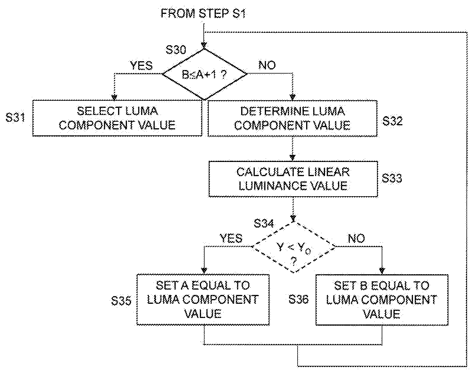
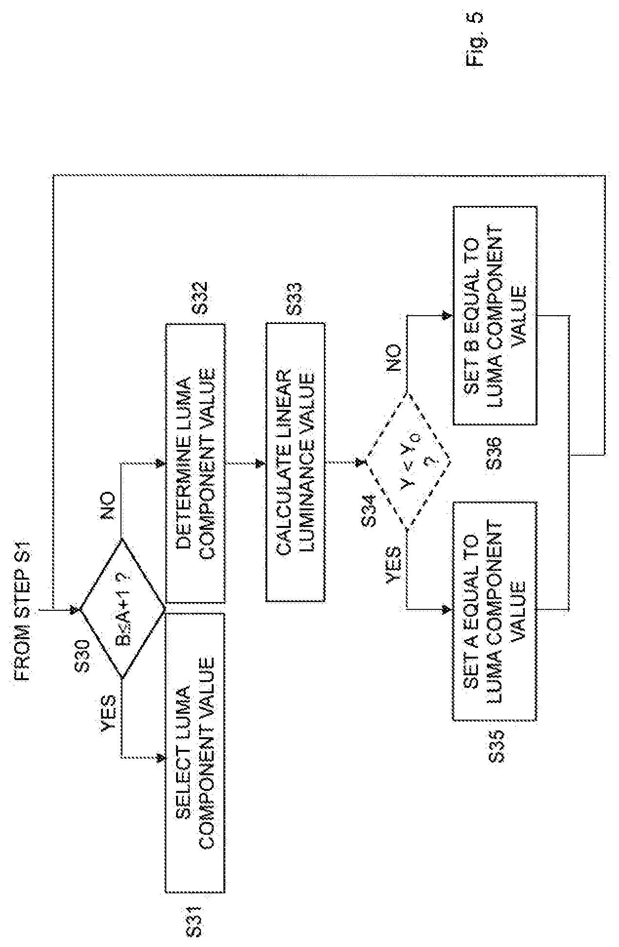
[0139] FIG. 5 schematically illustrates a flow chart of an embodiment involving performing a binary search. The method continues from step S1 in FIG. 1. In FIG. 5, the lower bound is represented by "A" and the upper bound is represented by "B". Optional step S30 comprises determining whether the upper bound is equal to or smaller than the lower bound plus one. This decision corresponds to checking whether the end of the binary search has been reached, i.e. arriving in a search interval of [p, p+1] for some value p. If the step S30 determines that the end of the binary search has been reached, the method continues to step S31. This step S31 comprises selecting the luma component value as either the upper bound or the lower bound. This is further described in connection with FIG. 6.
[0140] However, if the upper bound is larger than the lower bound plus one as determined in step S30, the method continues to step S32. Step S32 comprises determining a luma component value in the middle of an interval bounded by the lower bound and the upper bound. In a particular embodiment, this luma component value is determined as floor((lower bound+upper bound)/2). The method then continues to step S33, which comprises calculating a linear luminance value Y in the third color space based on the luma component value determined in step S32, the first chroma component value and the second chroma component value in the second color space.
[0141] An optional step S34 compares the calculated linear luminance value Y with the desired linear luminance component value Y.sub.o. If the calculated linear luminance value Y is smaller than the desired linear luminance component value Y.sub.o the method continues to step S35, otherwise the method continues to step S36.
[0142] Step S35 comprises setting the lower bound equal to the determined luma component value, whereas step S36 comprises setting the upper bound equal to the determined luma component value.
[0143] The method continues from step S35 or S36 to step S30. This means that the loop of steps S30, S32, S33, S34, S34, S35 or S36 halves the search interval.
[0144] The embodiments will speed up the binary search by determining an upper bound and/or a lower bound for the search interval, thereby potentially leading to a reduction of the number of cycles of the loop as compared to using the maximum allowable range for the luma component value.
[0145] This means that we do not need to set the upper bound b to 1023 and/or the lower bound a to 0 in the pseudo code for performing a binary search:
a=0 b=1023 [a, b]=performBinarySearch(a, b, Y.sub.o, Cb10 bit, Cr10bit, 10)
[0146] In clear contrast, we can convert Y'.sub.highest and/or Y'.sub.lowest to, in this example, a 10 bit integer and set b and/or a to that using
b=ceil(Y'10bit_highest)=ceil(4(219*Y'.sub.highest+16))
a=floor(Y'10bit_lowest)=floor(4(219*Y'.sub.lowest+16))
where ceil() rounds to the nearest larger integer and floor() rounds to the nearest smaller integer. In the above equations, we used the restricted range, which means that 64 maps to 0.0 and 940 maps to 1.0. If another range is wanted we need to adjust the equation. As an example, if we use the range [0, 1023] we can use
b=ceil(Y'.sub.10bit_highest)=ceil((1023*Y'.sub.highest))
a=floor(Y'.sub.10bit_lowest)=floor((1023*Y'.sub.lowest))
[0147] Assume in a first example, that the upper bound is determined for the luma component value. If the interval length b-a<512, we have saved ourselves one iteration. If b-a<256, we have saved two iterations, etc. If we only use an upper bound, we can, thus, instead use the following pseudo code:
TABLE-US-00002 a = 0 Y'.sub.highest.sub.--.sub.10bits = calcYpHighest( Yo, Cb10bit, Cr10bit ) b = min (1023, Y'.sub.highest.sub.--.sub.10bits ) if( b-a>512 ) N = 10 else if ( b-a>256 ) N = 9 else if ( b-a>128 ) N = 8 else if ( b-a>64 ) N = 7 else if ( b-a>32 ) N = 6 else if ( b-a>16 ) N = 5 else if ( b-a>8 ) N = 4 else if ( b-a>4 ) N = 3 else N = 2 end [a, b] = performBinarySearch( a, b, Y.sub.o, Cb10bit, Cr10bit, N ) Ya = calcY( a, Cb10bit, Cr10bit ) Yb = calcY( b, Cb10bit, Cr10bit ) e1 = ( Ya - Y.sub.o ).sup.2 e2 = ( Yb - Y.sub.o ).sup.2 if( e1 < e2 ) use Y' = a else use Y' = b end
[0148] Here, calcYpHighest performs the following actions:
TABLE-US-00003 Y'.sub.highest_10bits = calcYpHighest( Y.sub.0, Cb10bit, Cr10bit) { Y'.sub.highest = tf( Y.sub.0 ), return( ceil(4.0*(219.0*Y.sub.highest + 16)) ) }
[0149] Note that if we use the restricted interval [64, 940], we can set a=64 and b=min(940, Y'.sub.highest_10bits). In the above function we have assumed the interval is the full [0, 1023].
[0150] Assume in a second example, that the both the upper and lower bounds are determined for the luma component value. We can then change the pseudo code from
TABLE-US-00004 a = 0 Y'.sub.highest_10bits = calcYpHighest( Y', Cb10bit, Cr10bit ) b = min( 1023, Y'.sub.highest_10bits ) to Y.sub.lowest_10bits = calcYpLowest( Y.sub.0, Cb10bit, Cr10bit ) Y.sub.highest_10bits = calcYpHighest( Y.sub.0, Cb10bit, Cr10bit ) a = max( 0, Y'.sub.lowest_10bits ) b = min( 1023, Y'.sub.highest_10bits ) where calcYpLowest is described below: Y.sub.lowest_10bits = calcYpLowest( Y.sub.0, Cb10bit, Cr10bit ) { Cb = dClip( ( ( 1.0*Cb10bit ) / 4.0 - 128.0 ) / 224.0, -0.5, 0.5); Cr = dClip( ( ( 1.0*Cr10bit ) / 4.0 - 128.0 ) / 224.0, -0.5, 0.5); tf_var = tf(Y.sub.0); Y'.sub.lowest = tf_var - a13*Cr; Y'.sub.lowest = min( Y.sub.lowest, tf_var - a22*Cb - a23*Cr); Y'.sub.lowest = min(Y'.sub.lowest, tf_var - a32*Cb); Y'.sub.lowest_10bits = ( ceil( 4.0*( 219.13*Y'.sub.lowest + 16 ) ) ) end return (Y'.sub.lowest_10bits) }
[0151] An alternative version of calcYpHighest, which we call calcYpHighestAlternative can used:
TABLE-US-00005 Y'.sub.lowest_10bits = calcYpLowest( Y.sub.0, Cb10bit, Cr10bit ) Y'.sub.highest_10bits = calcYpHighestAlternative( Y.sub.0, Cb10bit, Cr10bit ) a = max( 0, Y'.sub.lowest_10bits ) b = min( 1023, Y'.sub.highest_10bits ) where calcYpHighestAlternative is described below: Y'.sub.highest_10bits = calcYpHighestAlternative(Y.sub.0, Cb10bit, Cr10bit) { Cb = dClip( ( ( 1.0*Cb10bit ) / 4.0 - 128.0 ) / 224.0, -0.5, 0.5); Cr = dClip( ( ( 1.0*Cr10bit ) / 4.0 - 128.0 ) / 224.0, -0.5, 0.5); tf_var = tf( Y.sub.0 ); Y'.sub.highest = tf_var - a13*Cr; Y'.sub.highest = max( Y.sub.highest, tf_var - a22*Cb - a23*Cr ); Y'.sub.highest = max( Y.sub.highest, tf_var - a32*Cb ); Y.sub.highest_10bits = ( floor( 4.0*( 219.0*Y.sub.highest + 16 ) ) ) return( Y'.sub.highest_10bits ) }
where floor(a) rounds the number a to the closest lower integer. This makes it possible to further decrease the size of the interval, thus, reducing the number of iterations needed and hence reducing the running time and complexity.
[0152] In yet an alternate embodiment, both calcYpHighest and calcYpHighestAlternative are used, and the tightest, i.e. lowest, bound is used:
calcYpHighestTightest(Y.sub.o,Cb10 bit,Cr10bit)=min(calcYpHighest(Y.sub.o,Cb10 bit,Cr10bit), calcYpHighestAlternative(Y.sub.o,Cb Obit,Cr10bit)).
[0153] This makes it possible to further decrease the size of the interval, thus, reducing the number of iterations needed and hence reducing the running time and complexity.
[0154] In an embodiment, the method comprises the additional steps S40 to S44 as shown in FIG. 6. These steps S40 to S44 illustrate a particular embodiment of step S31 shown in FIG. 5. Hence, the method continues from step S30 in FIG. 5 to step S40. This step S40 comprises calculating a first linear luminance value based on the lower bound and the first chroma component value and the second chroma component value in the second color space. Step S41 comprises calculating a first difference between the first linear luminance value and the desired linear luminance value. Step S42 correspondingly comprises calculating a second linear luminance value based on the upper bound and the first chroma component value and the second chroma component value in the second color space. The following step S43 comprises calculating a second difference between the second linear luminance value and the desired linear luminance value. Steps S40-S43 can be performed in any order or at least partly parallel as long as step S40 is performed prior to step S41 and step S42 is performed prior to step S43.
[0155] The method then continues to step S44, which comprises selecting the lower bound as the luma component value in the second color space if the first difference is smaller than the second difference and otherwise selecting the upper bound as the luma component value in the second color space.
[0156] The differences calculated in step S41 and S43 could be absolute differences |Y-Y.sub.o| or squared differences (Y-Y.sub.o).sup.2. The differences, such as absolute differences or squared differences, could be differences between a function of the first or second linear luminance value and a function of the desired linear luminance value. The function could, for instance, be the perceptual quantizer transfer function.
[0157] In this embodiment, the binary search, such as performed as described above in connection with FIG. 5, could output, two values, the lower bound and the upper bound. These two values correspond to a and b in the pseudo code: [a, b]=performBinarySearch(a, b, Y.sub.o, Cb10bit, Cr10bit, N)
[0158] The calculation of the first and second linear luminance values Ya, Yb are represented, in the pseudo code by the lines:
Ya=calcY(a,Cb10bit,Cr10bit)
Yb=calcY(b,Cb10bit,Cr10bit)
[0159] Thereafter these two differences or error values are calculated between the first or second linear luminance values and the desired linear luminance value Y.sub.o to see which of them results in the smallest difference:
e1=(Ya-Y.sub.o).sup.2
e2=(Yb-Y.sub.o).sup.2
[0160] In this example, the squared difference is calculated. In another embodiment, the absolute difference could be calculated. Then the luma component value is set equal to the lower bound or the upper bound based on a comparison of the calculated errors:
TABLE-US-00006 if( e1 < e2 ) use Y' = a else use Y' = b end
[0161] In the previous examples, going from equation 5 to equation 6 above we assumed that there was no clipping of the R', G' and B' variables. We will now further investigate how clipping affects this. We start by dividing up the clipping in step 2 into three steps:
R'=Y'+a13*Cr
G'=Y'+a22*Cb+a23*Cr
B'=Y'+a32*Cb
R'.sub.1=min(R',1)
G'.sub.1=min(G',1)
B'.sub.1=min(B',1)
R'.sub.01=max(R'1,0)
G'.sub.01=max(G'1,0)
B'.sub.01=max(B'1,0)
[0162] The first step calculates unclipped values, the second sets all values larger than 1 to 1, and the third step sets all values smaller than 0 to 0. Repeating equation 4 again:
Y.sub.result=w.sub.Rtf.sup.-1(R'.sub.01)+w.sub.Gtf.sup.-1(G'.sub.01)+w.s- ub.Btf.sup.-1(B'.sub.01) (equation 4)
[0163] Now the function tf.sup.-1(x) is not defined for negative values x, but it is easy to extend it to negative values. As an example, we can extend it so that tf.sup.-1(x)=0 if x<0. It is easy to see from FIG. 3 that the extended function is still convex. But with the extended function, there is no difference between that R'.sub.01 and R'.sub.1. Hence, Y.sub.result=w.sub.Rtf.sup.-1(R'.sub.1)+w.sub.Gtf.sup.-1(G'.sub.1)- +w.sub.Btf.sup.-1(B'.sub.1) where we have used boldface for tf.sup.-1(x) to signal that we use the extended version of the function. Since the extended function is still convex, we can use the convexity and write Y.sub.result=w.sub.Rtf.sup.-1(R'.sub.1)+w.sub.Gtf.sup.-1(G'.sub.1)+w.sub.- Btf.sup.-1(B'.sub.1).gtoreq.tf.sup.-1(w.sub.RR'.sub.1+w.sub.BB'.sub.1+w.su- b.GG'.sub.1).
[0164] Now assume we will use a Y' that is small enough so that none of the values R', G' or B' is larger than 1. In that case R'.sub.1=R', G'.sub.1=G' and B'.sub.1=B'. This means we can write Y.sub.result.gtoreq.tf.sup.-1(w.sub.RR'+w.sub.GG' +w.sub.BB') and continue with equation 6 above to calculate the highest possible Y' value Y'.sub.highest, Y'.sub.highest=tf(Y.sub.o).
[0165] We can now test this bounding value and see if it results in R', G' or B'-values higher than 1:
R'=Y'.sub.highest+a13*Cr
G'=Y'.sub.highest+a22*Cb+a23*Cr
B'=Y'.sub.highest+a32*Cb (equation 3b)
[0166] If one or more of R', G' and B' is larger than 1 in equation 3b, this indicates that the optimal value for Y', i.e. the Y' which will result in a linear Y value as close as possible to Y.sub.o, may also clip these values. In this case, the bound is not guaranteed to hold and it is safest not to say anything about the highest possible value, so we set b to 1023, or alternatively to 1019 or 940.
[0167] Actually, even if Y'.sub.highest does not cause any of R', G' and B' to exceed 1 in equation 3b, it is still theoretically possible that the optimal value for Y', when inserted into equation 3a would result in R', G' and B' values larger than 1. This is due to the fact that if the optimal value clips, then the derivation of Y'.sub.highest is no longer valid, and we may get a Y'.sub.highest that is too low, low enough for R', G' and B' not to clip in equation 3b. So in either case, we cannot be sure that Y'.sub.highest is a true bound for the optimal value for Y'.
[0168] However, in practice we have not been able to find a single combination of variables where the optimal Y' clips but Y'.sub.highest does not. In fact, it seems likely that if Y'.sub.highest does not result in R', G' and B' larger than one when inserted into equation 3b, then it is also a true bound for the optimal Y'.
[0169] To account for clipping against 1, it is therefore sufficient to test if equation 3b results in values larger than one. We therefore modify our function calcYpHighest(Y.sub.o) according to:
TABLE-US-00007 Y'.sub.highest_10bits = calcYpHighest( Y.sub.0, Cb10bit, Cr10bit) { Cb = dClip( ( ( 1.0*Cb10bit ) / 4.0 - 128.0)/ 224.0, -0.5, 0.5); Cr = dClip( ( ( 1.0*Cr10bit ) / 4.0 - 128.0)/ 224.0, -0.5, 0.5); Y'.sub.highest = tf( Y.sub.0 ); R' = Y'.sub.highest+ a13*Cr; G' = Y'.sub.highest + a22*Cb + a23*Cr; B' = Y'.sub.highest + a32*Cb; if( R' > 1 OR G' > 1 OR B' > 1 ) Y'.sub.highest_10bits = 1023; else Y'.sub.highest_10bits = ceil( 4.0*( 219.0*Y'.sub.highest + 16 ) ) end return( Y'.sub.highest_10bits ) }
[0170] In an alternative embodiment we use the other, more conservative upper bound to teste if the tighter upper bound can be used. Thus we first use the following pseudo code to calculate
TABLE-US-00008 Y'.sub.highest_conservative: Y'.sub.highest_conservative = calcYpHighestConservative(Y.sub.0, Cb10bit, Cr10bit) { Cb = dClip( ( ( 1.0*Cb10bit ) / 4.0 - 128.0 ) / 224.0, -0.5, 0.5); Cr = dClip( ( ( 1.0*Cr10bit ) / 4.0 - 128.0 ) / 224.0, -0.5, 0.5); tf_var = tf( Y.sub.0 ); Y'.sub.highest_conservative = tf_var - a13*Cr; Y'.sub.highest_conservative = max( Y'.sub.highest_conservative, tf_var - a22*Cb - a23*Cr ); Y'.sub.highest_conservative = max( Y'.sub.highest_conservative, tf_var - a32*Cb ); Y.sub.highest_conservative = min(Y'.sub.highest_conservative , 1.0); return( Y'.sub.highest_conservative ) }
[0171] Now, we can use this value to calculate the tighter bound safely:
TABLE-US-00009 Y'.sub.highest_10bits = calcYpHighestSafe( Y.sub.0, Cb10bit, Cr10bit, Y'.sub.highest_conservative ) { Cb = dClip( ( ( 1.0*Cb10bit ) / 4.0 - 128.0)/ 224.0, -0.5, 0.5); Cr = dClip( ( ( 1.0*Cr10bit ) / 4.0 - 128.0) / 224.0, -0.5, 0.5); Y'.sub.highest = tf( Y.sub.0 ); R' = Y'.sub.highest_conservative+a13*Cr; G' = Y'.sub.highest_conservative + a22*Cb + a23*Cr; B' = Y'.sub.highest_conservative + a32*Cb; if( R' > 1 OR G' > 1 OR B' > 1) Y'.sub.highest_10bits = ceil( 4.0*( 219.0*Y'.sub.highest_conservative + 16 ) ); else Y'.sub.highest_10bits = ceil( 4.0*( 219.0*Y'.sub.highest + 16 ) ) end return( min(Y'.sub.highest_10bits, 940) ) }
[0172] This way of calculating the upper bound is safe, since if the highest possible value for Y', which is Y'.sub.highest_conservative, does not clip against 1 for R, G and B, then Y' cannot clip either against 1 and it is, thus, safe to use the tighter bound Y'.sub.highest. However, if the upper bound Y'.sub.highest_conservative clips against 1 it may be the case that the optimal Y' also clips against 1, which in turn means that the tighter upper bound Y'.sub.highest may not be correct.
[0173] In practice, however, it is likely sufficient to do the clipping test using Y'.sub.highest instead of using Y'.sub.highest_conservative, as is done in calcYpHighest( ). This has two advantages. First, it is not necessary to calculate Y'.sub.highest_conservative to do the test, and second, since Y'.sub.highest<Y'.sub.highest_conservative it will also result in fewer instances where the looser bound is used, which provides a tighter bound in more cases thus avoiding iterations.
[0174] Note that it may not be free to execute calcYpHighest(). Therefore it makes sense to make it as quick as possible. One idea is to create a lookup table (LUT) for the calculation of the transfer function tf(), which is otherwise likely the slowest part of calcYoHighest( ). Since this LUT is one-dimensional, it will not take up a lot of space. As an example, if 1024 values are used in the LUT, and each value is a double, taking 8 bytes, only 8 kB will be necessary for the LUT.
[0175] In order to improve the accuracy of the LUT, it may be advantageous to fetch the two nearest LUT values and perform linear interpolation between them. The LUT can also be constructed so that it is conservative--the linear approximation of the transfer function can be made to always be above the transfer function, instead of being as close as possible to the transfer function. This way we are assured the Y'.sub.highest will be a true bound, something which would not be possible if some interpolated LUT values were below the actual transfer function. Another way to get a conservative value is to not use linear interpolation, but always round up. As an example, if the value of Y.sub.o indicates that we should look for a value that is between the LUT position 114 and 115, we can always take the value 115. Since the transfer function is monotonically increasing, all the values of the transfer function between 114 and 115 must be smaller than the LUT value in position 115.
[0176] As an example, if we have a LUT of size 1023, we may exchange the line
Y'.sub.highest=tf(Y.sub.o);
with
Y'.sub.highest=TF_LUT[ceil(Y.sub.o*1023)];
[0177] where ceil rounds up to the nearest integer.
[0178] Likewise, when we are using the lower bound, we may use a LUT conservative the other way, i.e. all the interpolated values from the LUT are always lower or equal to the actual value of the transfer function for that point.
[0179] FIG. 7 illustrates when combined with FIG. 1 a method of encoding a pixel in a picture. The method comprises pre-processing the pixel in steps S1 and S2 according to any of the embodiments to obtain a luma component value in the second color space for the pixel. The method then continues to step S3 in FIG. 7. This step S3 comprises encoding the luma component value, a subsampled first chroma component value and a subsampled second chroma component value in the second color space.
[0180] The two subsampled chroma component values are the Cb`Cr` values subsampled into the 4:2:0 or 4:2:2 format. Subsampling can be performed according to known subsampling techniques. For instance, a filtering operation or a nearest neighbor operation can be used. An example of subsampling technique that can be used according to the embodiments is disclosed in section B.1.5.5 Chroma downsampling from 4:4:4 to 4:2:0 in document [5].
[0181] The output of the pre-processing, i.e. Y'Cb'Cr', such as in the 4:2:0 or 4:2:2 format, is then input to a video encoder, such as a H.264 video encoder, a High Efficiency Video Encoder (HEVC) or H.265 video encoder, or another video encoder. The encoding as performed by the video encoder can include traditional video encoding steps, such as inter prediction, intra prediction, mode decision, transformation of residual, quantization and encoding of the transformed and quantized residuals, such as in an entropy encoder.
[0182] An advantage of the pre-processing of the embodiments is that it can be applied to any video or picture encoding process without the need for performing any adjustments in the video or picture encoder or any adjustments in the corresponding video or picture decoder.
[0183] The pre-processing of pixels in pictures, such as of a video sequence, may also be used in other applications besides video encoding. For instance, the embodiments can be used as a pre-processing that is applied before transferring video over an interface, such as high-definition multimedia interface (HDMI), DisplayPort or Thunderbolt. For example, in HDMI 2.0a the only way to convey 4K resolution at 50 or 60 frames per second (fps) is to use 4:2:0 or 4:2:2 YCbCr subsampling. If the video data is in full chroma sampling format (4:4:4) then a subsampling pre-processing step must be applied before sending the video data over the HDMI cable. The 4:2:0 or 4:2:2 video data is then transferred over the interface without further compression. By applying the pre-processing of the embodiments, the video quality is improved compared to conventional 4:2:0 or 4:2:2 subsampling in the non-linear domain, i.e. subsampling of Cb`Cr` values.
[0184] According to an embodiment, a method is provided for an encoder or for a pre-process to an encoder, or for a conversion process, for calculating an upper bound for a suitable Y' value referred to as Y'-value to be used for HDR encoding. The suitable Y'-value can be thought of as a corrected Y' value compared to the Y' value traditional processing would give. The suitable Y' value will result in a linear luminance closer to the desired linear luminance Y.sub.o. Further the upper bound of the Y'-value, i.e. Y'.sub.highest, is determined as a function of the desired linear luminance Y.sub.o. In more detail, the upper bound Y'.sub.highest may be calculated as Y'.sub.highest=tf(Y.sub.o), wherein tf is a concave transfer function.
[0185] The desired linear luminance is calculated as Y.sub.o=w.sub.R*R.sub.o+w.sub.G*G.sub.o+w.sub.B*B.sub.o, where (R.sub.o, G.sub.o, B.sub.o) are the original linear RGB values for the pixel.
[0186] The concave transfer function can be any concave transfer function defined on the interval [0, 1], such as a normal gamma y=x.sup.(1/2.2).
[0187] Further a lower bound of the Y'-value, Y'.sub.lowest, is determined based on a function of the desired linear luminance Y.sub.o. In more detail, the lower bound of the Y'-value, Y'.sub.lowest, may be determined based on a function of tf(Y.sub.o), where tf( ) is a monotonously increasing transfer function. In yet more detail, the lower bound of the Y'-value, Y'.sub.lowest, may be determined as Y'.sub.lowest=min(tf(Y.sub.o)-a.sub.13*Cr, tf(Y.sub.o)-a22*Cb-a23*Cr, tf(Y.sub.o)-a32*Cb, 0).
[0188] It is possible to only determine the upper bound or only the lower bound or both the lower and the upper bounds.
[0189] Thus, according to a first aspect of the present invention a method is provided for an encoder, for a pre-process to an encoder, or for a conversion process, for calculating at least one bound for a suitable Y' value referred to as Y'-value to be used for HDR encoding, display, or further processing. The at least one bound is determined as or based on a function of a desired linear luminance Y.sub.o, wherein the function is a transfer function.
[0190] The proposed solution allows a faster conversion from RGB 4:4:4 to Y'CbCr 4:2:0 than previous art.
[0191] The proposed solution allows a conversion from RGB 4:4:4 to Y'CbCr 4:2:0 that uses less memory than previous art.
[0192] The proposed solution allows a conversion from RGB 4:4:4 to Y'CbCr 4:2:0 that is of a higher quality than previous art.
[0193] In the foregoing, embodiments have been described with regard to Y' as luma component value, CbCr as chroma component values and Y'CbCr as the second color space.
[0194] The embodiments are, however, not limited thereto. ICtCp is an alternative color space, in which the I value carries luma information and the CtCp values carry chroma information. In an embodiment, LMS values in the LMS color space can be obtained from RGB values and a color transform according to below:
L=(1688*R+2146*G+262*B)/4096
M=(683*R+2951*G+462*B)/4096
S=(99*R+309*G+3688*B)/4096
[0195] A transfer function, such as the inverse of EOTF.sub.PQ, can then be applied to the LMS values in order to obtain non-linear L'M'S' values. Finally, a color transform is applied to these L'M'S' value to obtain the ICtCp values:
I=0.5*L'+0.5*M'
Ct=(6610*L'-13613*M'+7003*S')/4096
Cp=(17933*L'-17390*M'-543*S')/4096
[0196] The embodiments can then be applied to this case with I representing luma component value and CtCp representing the first and second chroma component values and ICtCp being the second color space.
[0197] Another aspect of the embodiments relates to a device for pre-processing a pixel in a picture. The device is configured to determine at least one bound for a luma component value of the pixel in a second color space based on a function of a desired linear luminance value of the pixel in a third color space, wherein the function is a transfer function. The device is also configured to select a luma component value in the second color space for the pixel within an interval comprising multiple luma component values in the second color space and bounded by the at least one bound, wherein a color of the pixel is represented by the luma component value, a first chroma component value and a second chroma component value in the second color space.
[0198] In an embodiment, the device is configured to determine the desired linear luminance value based on a linear color of the pixel in a first color space.
[0199] In an embodiment, the device is configured to determine an upper bound for the luma component value and for the interval based on, preferably as, tf(Y.sub.o). tf() is a concave transfer function and Y.sub.o denotes the desired linear luminance value.
[0200] In another embodiment, the device is configured to determine an upper bound for the luma component value and for the interval as a maximum of tf(Y.sub.o)-a.sub.13Cr, tf(Y.sub.o)-a.sub.22Cb-a.sub.23Cr and tf(Y.sub.o)-a.sub.32Cb. tf() is a monotonously increasing transfer function, Y.sub.o denotes the desired linear luminance value, Cb denotes the first chroma component value in the second color space, Cr denotes the second chroma component value in the second color space, and the constants a.sub.13=1.57480, a.sub.22=-0.18733, a.sub.23=-0.46813 and a.sub.32=1.85563 for Rec.709 and a.sub.13=1.47460, a.sub.22=-0.16455, a.sub.23=-0.57135 and a.sub.32=1.88140 for BT.2020.
[0201] In a further embodiment, the device is configured to determine a first bound as tf(Y.sub.o). tf() is a concave transfer function and Y.sub.o denotes the desired linear luminance value. The device is also configured to determine, if a test value calculated based on the first bound is larger than one, a second bound as a maximum of tf(Y.sub.o)-a.sub.13Cr, tf(Y.sub.o)-a.sub.22Cb-a.sub.23Cr and tf(Y.sub.o)-a.sub.32Cb. tf() is a monotonously increasing transfer function, Cb denotes the first chroma component value in the second color space, Cr denotes the second chroma component value in the second color space, and the constants a.sub.13=1.57480, a.sub.22=-0.18733, a.sub.23=-0.46813 and a.sub.32=1.85563 for Rec.709 and a.sub.13=1.47460, a.sub.22=-0.16455, a.sub.23=-0.57135 and a.sub.32=1.88140 for BT.2020. The device is further configured to select an upper bound for the luma component value and for the interval as the second bound if the test value is larger than one and otherwise select the first bound.
[0202] In an embodiment, the device is configured to determine a lower bound for the luma component value and for the interval based on, preferably as, tf(Y.sub.o). tf() is a monotonously increasing transfer function and Y.sub.o denotes the desired linear luminance value.
[0203] In a particular embodiment, the device is configured to determine the lower bound as a minimum of tf(Y.sub.o)-a.sub.13Cr, tf(Y.sub.o)-a.sub.22Cb-a.sub.23Cr and tf(Y.sub.o)-a.sub.32Cb. Cb denotes the first chroma value in the second color space, Cr denotes the second chroma value in the second color space, and the constants a.sub.13=1.57480, a.sub.22=-0.18733, a.sub.23=-0.46813 and a.sub.32=1.85563 for Rec.709 and a.sub.13=1.47460, a.sub.22=-0.16455, a.sub.23=-0.57135 and a.sub.32=1.88140 for BT.2020.
[0204] In an embodiment, the device is configured to select, within the interval, a luma component value that minimizes a difference between the desired linear luminance value and a linear luminance value in the third color space calculated based on the luma component value, the first chroma component value and the second chroma component value in the second color space.
[0205] In an embodiment, the device is configured to perform a binary search to select the luma component value within the interval.
[0206] In a particular embodiment, the device is configured to perform, as long as an upper bound for said luma component value is larger than a lower bound for said luma component value plus one, the following operations. The device is configured to determine a luma component value in the middle of an interval bounded by said lower bound and said upper bound. The device is also configured to calculate a linear luminance value in said third color space based on said determined luma component value, said first chroma component value and said second chroma component value in said second color space. The device is additionally configured to set said lower bound equal to said determined luma component value if said calculated linear luminance value is smaller than said desired linear luminance value or otherwise set said upper bound equal to said determined luma component value. Once the device determines that the upper bound is no longer larger the lower bound plus one, the device is configured to select said luma component value as said lower bound or said upper bound.
[0207] In an embodiment, the device is additionally configured to calculate a first linear luminance value based on the lower bound, the first chroma component value and the second chroma component value in the second color space. The device is also configured to calculate a first difference between the first linear luminance value, or a function thereof, and the desired linear luminance value, or the function thereof. The device is further configured to calculate a second linear luminance value based on the upper bound, the first chroma component value and the second chroma component value in the second color space. The device is additionally configured to calculate a second difference between the second linear luminance value, or the function thereof, and the desired linear luminance value, or the function thereof. The device is further configured to select the lower bound as the luma component value in the second color space if the first difference is smaller than the second difference and otherwise selecting the upper bound as the luma component value in the second color space.
[0208] According to a second aspect of the present invention an arrangement or device 100 is provided, see FIG. 8. The arrangement or device 100 is exemplified by an encoder, a pre-process to an encoder, or a conversion process, for calculating at least one bound for a suitable Y' value referred to as the Y'-value to be used for HDR encoding, display or further processing is provided. The arrangement or device 100 is configured to determine the at least one bound based on a function of a desired linear luminance Y.sub.o, wherein the function is a transfer function.
[0209] Hence the arrangement or device 100 may comprise a determining unit 101 for determining the at least one bound based on a function of a desired linear luminance Y.sub.o, wherein the function is a transfer function.
[0210] Moreover, the arrangement or device 100 and the determining unit 101 may be configured to do the determination according to any of the embodiments below or a combination thereof.
[0211] According to one embodiment, the at least one bound is an upper bound and the transfer function is a concave transfer function.
[0212] According to a further embodiment the at least one bound is a lower bound and the transfer function is a monotonously increasing transfer function.
[0213] The arrangement or device 100 may in addition to the determining unit 101 further comprise an encoding unit or encoder 102 and an input unit 103 configured to receive the video to be encoded and an output unit 103 configured to output an encoded bitstream. The encoder 102 is preferably arranged for encoding the luma component value, the subsampled first chroma component value and the subsampled second chroma component value in the second color space.
[0214] The input unit 103 could be in the form of a general input unit, in particular in the case of a wired connection to external devices. Alternatively, the input unit 103 could be in the form of a receiver or transceiver, in particular in the case or a wireless connection to external devices. Correspondingly, the output unit 104 could be in the form of a general output unit, in particular in the case of a wired connection to external devices. Alternatively, the output unit 104 could be in the form of a transmitter or transceiver, in particular in the case or a wireless connection to external devices.
[0215] The input unit 103 may connected to the determining unit 103 and the encoding unit 102. The encoding unit 102 may be connected to the determining unit 101 and to the output unit 104 to forward the encoded bitstream to a decoder.
[0216] According to a further aspect, the device 110 comprises a processor 111 and a memory 112 comprising instructions executable by the processor 112, see FIG. 9. The processor 111 is operative to determine the at least one bound for the luma component value. The processor 111 is also operative to select the luma component value in the second color space for the pixel within the interval.
[0217] In an embodiment, the processor 111 is operative to determine the at least one bound based on a function of a desired linear luminance Y.sub.o, wherein the function is a transfer function.
[0218] The device 110 may optionally comprise an input unit 113 and an output unit 114. In such a case, the input unit 113 is configured to receive pictures of a video sequence to the pre-processed by the device 110 and the processor 111 according to the instructions stored in the memory 112. The output unit 114 is then configured to output the pre-processed pictures, or if the device 110 additionally is configured to encode the pre-processed pictures, an encoded bitstream representing an encoded version of the pictures of the video sequence.
[0219] Yet another aspect of the embodiments relates to a device 110 for encoding a pixel in a picture. The device 110 comprises a processor 111 and a memory 112 comprising instructions executable by the processor 111. The processor 111 is operative to determine at least one bound for a luma component value of the pixel in a second color space based on a function of a desired linear luminance value of the pixel in a third color space. The function is a transfer function. The processor 111 is also operative to select a luma component value in the second color space for the pixel within an interval comprising multiple luma component value sin the second color space and bounded by the at least one bound. The processor 111 is further operative to encode the luma component value, a subsampled first chroma component value and a subsampled second chroma component value in the second color space.
[0220] Alternatively, at least some of the steps, functions, procedures, modules and/or blocks described herein may be implemented in software such as a computer program 240 for execution by suitable processing circuitry such as one or more processors or processing units 210 of a user equipment 200, see FIG. 10.
[0221] Examples of processing circuitry includes, but is not limited to, one or more microprocessors, one or more Digital Signal Processors (DSPs), one or more Central Processing Units (CPUs), video acceleration hardware, and/or any suitable programmable logic circuitry such as one or more Field Programmable Gate Arrays (FPGAs), or one or more Programmable Logic Controllers (PLCs).
[0222] It should also be understood that it may be possible to re-use the general processing capabilities of any conventional device or unit in which the proposed technology is implemented. It may also be possible to re-use existing software, e.g. by reprogramming of the existing software or by adding new software components.
[0223] In a particular embodiment, the processor 210 is operative, when executing the instructions stored in the memory 220 to perform the above described operations. The processor 210 is thereby interconnected to the memory 220 to enable normal software execution.
[0224] In one example, at least some of the steps, functions, procedures, modules and/or blocks described herein are implemented in a computer program 240, which is loaded into the memory 220 for execution by processing circuitry including one or more processors 210. The processor 210 and memory 220 are interconnected to each other to enable normal software execution. A communication circuitry 230 is also interconnected to the processor 210 and/or the memory 220 to enable input and/or output of video data.
[0225] In an embodiment, the computer program 240 comprises instructions, which when executed by a processor 210, cause the processor 210 to determine at least one bound for a luma component value of the pixel in a second color space based on a function of a desired linear luminance value of the pixel in a third color space. The function is a transfer function. The processor 210 is also caused to select a luma component value in the second color space for the pixel within an interval comprising multiple luma component value sin the second color space and bounded by the at least one bound.
[0226] In an embodiment, the computer program 240 further comprises instructions, which when executed by the processor 210, cause the processor 210 to encode the luma component value, a subsampled first chroma component value and a subsampled second chroma component value in the second color space.
[0227] The user equipment 200 can be any device or apparatus that can receive and process video data. For instance, the user equipment 200 could be a computer, either stationary or portable, such as laptop, a smart phone, a tablet, a set-top box, etc.
[0228] The term `processor` should be interpreted in a general sense as any system or device capable of executing program code or computer program instructions to perform a particular processing, determining or computing task.
[0229] The processing circuitry including one or more processors is thus configured to perform, when executing the computer program, well-defined processing tasks such as those described herein.
[0230] The processing circuitry does not have to be dedicated to only execute the above-described steps, functions, procedure and/or blocks, but may also execute other tasks.
[0231] The proposed technology also provides a carrier 250 comprising the computer program 240. The carrier 250 is one of an electronic signal, an optical signal, an electromagnetic signal, a magnetic signal, an electric signal, a radio signal, a microwave signal, or a computer-readable storage medium.
[0232] By way of example, the software or computer program 240 may be realized as a computer program product, which is normally carried or stored on a computer-readable medium 250, preferably non-volatile computer-readable storage medium 250. The computer-readable medium may include one or more removable or non-removable memory devices including, but not limited to a Read-Only Memory (ROM), a Random Access Memory (RAM), a Compact Disc (CD), a Digital Versatile Disc (DVD), a Blue-ray disc, a Universal Serial Bus (USB) memory, a Hard Disk Drive (HDD) storage device, a flash memory, a magnetic tape, or any other conventional memory device. The computer program 240 may thus be loaded into the operating memory of a computer or equivalent processing device, represented by the user equipment 200 for execution by the processor 210 thereof.
[0233] The flow diagram or diagrams presented herein may therefore be regarded as a computer flow diagram or diagrams, when performed by one or more processors. A corresponding device may be defined as a group of function modules, where each step performed by the processor corresponds to a function module. In this case, the function modules are implemented as a computer program running on the processor. Hence, the device may alternatively be defined as a group of function modules, where the function modules are implemented as a computer program running on at least one processor.
[0234] The computer program residing in memory may thus be organized as appropriate function modules configured to perform, when executed by the processor, at least part of the steps and/or tasks described herein. An example of such function modules is illustrated in FIG. 11.
[0235] FIG. 11 is a schematic block diagram of a device 120 with function modules. The device 120 is, in an embodiment, a device for pre-processing a picture. The device 120 comprises a determining unit 121 for determining at least one bound for a luma component value of the pixel in a second color space based on a function of a desired linear luminance value of the pixel in a third color space. The function is a transfer function. The device 120 also comprises a selector 122 for selecting a luma component value in the second color space for the pixel within an interval comprising multiple luma component value sin the second color space and bounded by the at least one bound.
[0236] In another embodiment, the device 120 is a device for encoding a pixel in a picture. The device 120 comprises a determining unit 121 for determining at least one bound for a luma component value of the pixel in a second color space based on a function of a desired linear luminance value of the pixel in a third color space. The function is a transfer function. The device 120 also comprises a selector 122 for selecting a luma component value in the second color space for the pixel within an interval comprising multiple luma component value sin the second color space and bounded by the at least one bound. The device 120 further comprises an encoder 123 for encoding the luma component value, a subsampled first chroma component value and a subsampled second chroma component value in the second color space.
[0237] A further aspect of the embodiments relates to a user equipment comprising a device according to the embodiments, such as illustrated in any of FIG. 8, 9 or 11. The user equipment is selected from a group consisting of a computer, either stationary or portable, a laptop, a smart phone, a tablet, a set-top box, etc.
[0238] Yet another aspect of the embodiments relates to a signal representing an encoded version of a pixel in a picture. The encoded version comprises an encoded version of two subsample dchroma component values in a second color format and an encoded version of a luma component value in the second color format obtained according to any of the embodiments. In an embodiment, the signal is one of an electronic signal, an optical signal, an electromagnetic signal, a magnetic signal, an electric signal, a radio signal and a microwave signal.
[0239] It is becoming increasingly popular to provide computing services, such as hardware and/or software, in network devices, such as network nodes and/or servers, where the resources are delivered as a service to remote locations over a network. By way of example, this means that functionality, as described herein, can be distributed or re-located to one or more separate physical nodes or servers. The functionality may be re-located or distributed to one or more jointly acting physical and/or virtual machines that can be positioned in separate physical node(s), i.e. in the so-called cloud. This is sometimes also referred to as cloud computing, which is a model for enabling ubiquitous on-demand network access to a pool of configurable computing resources such as networks, servers, storage, applications and general or customized services.
[0240] FIG. 12 is a schematic diagram illustrating an example of how functionality can be distributed or partitioned between different network devices 300, 301, 302 in a general case. In this example, there are at least two individual, but interconnected network devices 300, 301, which may have different functionalities, or parts of the same functionality, partitioned between the network devices 300, 301. There may be additional network devices 302 being part of such a distributed implementation. The network devices 300, 301, 302 may be part of the same wireless communication system, or one or more of the network devices may be so-called cloud-based network devices located outside of the wireless communication system.
[0241] FIG. 13 is a schematic diagram illustrating an example of a wireless communication system, including an access network 1 and/or a core network 2 and/or an Operations and Support System (OSS) 3 in cooperation with one or more cloud-based network devices 300. The figure also illustrates a network node 4 of the access network 1 and a user equipment 5 according to the embodiments.
[0242] Annex A
[0243] This Annex A provides proof of generalization of convex functions to three variables: Directly from the definition of a convex function, we have that (A1) holds:
f(tx.sub.1+(1-t)x.sub.2).ltoreq.tf(x.sub.1)+(1-t)f(x.sub.2) (A1)
[0244] This can be generalized to three values. Assume x.sub.1, x.sub.2 and x.sub.3 are three values, and that we have three values w.sub.1, w.sub.2 and w.sub.3 such that w.sub.1+w.sub.2+w.sub.3=1. We now examine the following expression
f(w.sub.1x.sub.1+w.sub.2x.sub.2+w.sub.3x.sub.3) (A2)
by introducing a new variable x.sub.3',
x 3 ' = w 1 x 1 + w 2 x 2 ( 1 - w 3 ) . ( A3 ) ##EQU00001##
We can rewrite equation (A3) as
w.sub.1x.sub.1+w.sub.2x.sub.2=(1-w.sub.3)x'.sub.3 (A4)
and insert into (A1), which will yield
f((1-w.sub.3)x'.sub.3+w.sub.3x.sub.3).ltoreq.(1-w.sub.3)f(x'.sub.3)+w.su- b.3f(x.sub.3). (A5)
[0245] Here the inequality is just due to the convexity of f(x) following (A1). We can now put the value for x'.sub.3 back into the right hand side of the equation, and using the fact that (1-w.sub.3)=w.sub.1+w.sub.2 we get
f ( w 1 x 1 + w 2 x 2 + w 3 x 3 ) .ltoreq. ( w 1 + w 2 ) f ( w 1 x 1 + w 2 x 2 w 1 + w 2 ) + w 3 f ( x 3 ) = ( A6 ) = ( w 1 + w 2 ) f ( w 1 w 1 + w 2 x 1 + w 2 w 1 + w 2 x 2 ) + w 3 f ( x 3 ) . ( A7 ) ##EQU00002##
[0246] Setting
t = w 1 w 1 + w 2 , ##EQU00003##
we get that
( 1 - t ) = ( 1 - w 1 w 1 + w 2 ) = ( w 1 + w 2 w 1 + w 2 - w 1 w 1 + w 2 ) = w 2 w 1 + w 2 ##EQU00004##
and we can rewrite the first part of equation (A7) as
(w.sub.1+w.sub.2)f(tx.sub.1+(1-t)x.sub.2)+w.sub.3f(x.sub.3). (A8)
[0247] By again making use of (A1), we get
(w.sub.1+w.sub.2)f(tx.sub.1+(1-t)x.sub.2)+w.sub.3f(x.sub.3)(w.sub.1+w.su- b.2)[tf(x.sub.1)+(1-t)f(x.sub.2)]+w.sub.3f(x.sub.3). (A9)
[0248] Now putting back our value for t and (1-t) we get
( w 1 + w 2 ) [ w 1 w 1 + w 2 f ( x 1 ) + w 2 w 1 + w 2 f ( x 2 ) ] + w 3 f ( x 3 ) , ( A10 ) ##EQU00005##
which equals
w.sub.1f(x.sub.1)+w.sub.2f(x.sub.2)+.sub.3f(x.sub.3) (A11)
and we have therefore just proven that
f(w.sub.1x.sub.1+w.sub.2x.sub.2+w.sub.3x.sub.3).ltoreq.w.sub.1f(x.sub.1)- +w.sub.2f(x.sub.2)+w.sub.3f(x.sub.3) (A12)
if f(x) is convex.
[0249] Annex B
[0250] This Annex B describes the function performBinarySearch in pseudo code below:
TABLE-US-00010 [a_out, b_out] = performBinarySearch( a, b, Y.sub.0, Cb10bit, Cr10bit, N) { // First convert from integer representation to double Cb_double = dClip( ( ( 1.0*Cb10bit ) / 4.0 - 128.0 ) / 224.0, -0.5, 0.5); Cr_double = dClip( ( ( 1.0*Cr10bit ) / 4.0 - 128.0 ) / 224.0, -0.5, 0.5); convertFromYprimeToYlin2020( Ya, Cb_double, Cr_double, a); convertFromYprimeToYlin2020( Yb, Cb_double, Cr_double, b); // Now search for the best Y', denoted Yprime or Yp herein; for( int gg = 0; gg<N; gg++) { // First calculate midpoint Yp_mid = (a + b + 1) >> 1; // Convert new midpoint to linear RGB Ymid = convertFromYprimeToYlin2020( Yp_mid, Cb_double, Cr_double); // Now, if Ymid is smaller than the correct one, we should increase Y', hence mid is the new // low. Otherwise, mid is the new high. if( Ymid < Yo ) { a = Yp_mid; Ya = Ymid; } else { b = Yp_mid; Yb = Ymid; } } a_out = a; b_out = b; } and where convertFromYprimeToYlin2020 is defined as [Ylin] = convertFromYprimeToYlin2020( Yp, Cb_double, Cr_double ) { // First convert from integer representation to double Yp_double = ( ( 1.0*Yp ) / 4.0 - 16.0 ) / 219.0; // Now convert to RGB RGB_prime_pix[0] = dClip( Yp_double + 1.47460*Cr_double, 0, 1 ); RGB_prime_pix[1] = dClip( Yp_double - 0.16455*Cb_double - 0.57135*Cr_double, 0, 1); RGB_prime_pix[2] = dClip( Yp_double + 1.88140*Cb_double, 0, 1 ); // Convert back to linear light using linear approximation of LUT for( cc = 0; cc<3; cc++ ) RGB_pix[cc] = pq_eotf_jas( RGB_prime_pix[cc] ); // Finally, calculate the Y of XYZ from the linear RGB: Ylin = 0.262700 * RGB_pix[0] + 0.677998 * RGB_pix[1] + 0.059302 * RGB_pix[2]; }
[0251] Similar functions are available for the BT.709 color space, with different constants.
[0252] In the above function we have used a transfer function from ST.2084, here named pq_eotf_jas( ). It is reproduced here for the convenience of the reader:
pq_eotf _jas ( V ) = ( max [ ( V 1 / m - c 1 ) , 0 ] c 2 - c 3 V 1 / m ) 1 / n ##EQU00006## n = 2610 4096 .times. 1 4 .apprxeq. 0.15930176 ##EQU00006.2## m = 2523 4096 .times. 128 = 78.84375 ##EQU00006.3## c 1 = c 3 - c 2 + 1 = 3424 4096 = 0.8359375 ##EQU00006.4## c 2 = 2413 4096 .times. 32 = 18.8515625 ##EQU00006.5## c 3 = 2392 4096 .times. 32 = 18.6875 ##EQU00006.6##
[0253] Typically one says that the inverse of the EOTF function is the transfer function, hence
[0254] Typically one says that the inverse of the EOTF function is the transfer function, hence
tf(x)=pq_eotf_jas.sup.-1(x), and tf.sup.-1(x)=pq_eotf_jas(x).
[0255] Annex C
[0256] The present Annex C comprises a description of the Ajusty method that can be used according to the embodiments in order to derive a non-linear luma component value in the second color space.
[0257] A combination of a highly non-linear transfer function, 4:2:0 or 4:2:2 subsampling and non-constant luminance ordering gives rise to severe artifacts in saturated colors. An example is described in Annex B, where changes between two colors of similar luminance can result in a reconstructed image with very different luminances.
[0258] In a digital video signal, each component of a sample, i.e. pixel, is represented by an integer or floating point value. A display, such as screen, TV or monitor, that renders the video omits optical lights based on the digital values of the video signal. The function that translates the digital value V to optical light Y is the Electro-Optical-Transfer-Function (EOTF). Traditionally the EOTF has been expressed as an exponential function called a gamma function where the gamma y is the exponent value. This is typically 2.4 (but can also be other values): Y=V.sup..gamma..
[0259] Using a gamma function works well for low luminance signals but when the luminance goes above 100 nits (cd/m.sup.2) the gamma function is not well aligned with the contrast sensitivity of the human visual system. Therefore transfer functions that are more non-linear are defined, e.g.:
Y = L p ( max [ ( V 1 / m - c 1 ) , 0 ] c 2 - c 3 V 1 / m ) 1 / n n = 2610 4096 .times. 1 4 .apprxeq. 0.15930176 m = 2523 4096 .times. 128 = 78.84375 c 1 = c 3 - c 2 + 1 = 3424 4096 = 0.8359375 c 2 = 2413 4096 .times. 32 = 18.8515625 c 3 = 2392 4096 .times. 32 = 18.6875 L p = 10000 c d m 2 ( equation C1 ) ##EQU00007##
[0260] This transfer function is more non-linear than the gamma function in the sense that the maximum value of its first derivative over the range from 0 to 1 is larger than that of the gamma function.
[0261] Chroma subsampling is typically done before compression as an initial step to reduce the amount of data. In 4:2:2 the chroma signal is reduced to half the resolution in the vertical direction. In 4:2:0 the chroma signal is reduced to half the resolution in both the vertical direction and the horizontal direction. This is typically done with some filtering operation to get a good quality signal but can also be done using nearest neighbor.
[0262] In order to display a 4:2:0 or 4:2:2 video, a decoder performs upsampling of the chroma signal, which can be done using bilinear filters or longer filters.
[0263] However, a combination of a highly non-linear transfer function, 4:2:0 or 4:2:2 subsampling and non-constant luminance ordering gives rise to severe artifacts to the video data, in particular for saturated colors, i.e. colors close to the color gamut edge.
[0264] There are several ways to get around this problem. One ways is to not use 4:2:0 or 4:2:2 subsampling, but use 4:4:4 instead. That, however, is expensive, since 4:2:0 halves the number of bits prior to compression, whereas 4:2:2 reduces the number of bits to two-thirds. Another way is to not use a highly non-linear transfer function. However, that means that it is hard to represent content of very high peak brightness without having banding in dark regions. A third way is to use constant luminance, i.e. apply the transfer function after conversion to the CIE1931 XYZ color space. However, such a solution is not aligned with common practice within the broadcasting industry and might in some scenarios be difficult and expensive to realize.
[0265] A typical compression chain is described below. The incoming linear light pixel (R, G, B) ranging from 0 to 10,000 is first fed to the transfer function, which results in a new pixel (R', G', B') between 0 and 1. After this, the pixel undergoes color transform resulting in Y'Cb'Cr'. Then the Cb` and Cr` components are subsampled to 4:2:0.
[0266] After decompression, the 4:2:0 sequences are upsampled to 4:4:4 again, inverse color space conversion gives (R', G', B') and finally inverse transfer function gives back the linear light pixel (R, G, B) that can be output on a monitor.
[0267] The trouble comes from the fact that the Cb` and Cr` components are interpolated, whereas the Y' component is not. Hence there can be a sharp shift in the Y' component in a pixel, but the Cb` and Cr` component cannot follow, since they are interpolated. For some colors, especially saturated colors, the result is a pixel of completely wrong intensity, and it is clearly visible.
[0268] It is proposed to change the Y' component in these cases so that the tuple (Y' Cb' Cr') generated from the interpolated colors is not so different from the original. Ideally the difference would be so small that it is not noticeable.
[0269] Basically it emanates to realizing that the Cb` and Cr` components are false, and then make also the Y' component false so that the (Y' Cb' Cr') are closer to the true colors. In other words, by introducing an error in Y' we can compensate for the errors already existing in Cb` and Cr` to come closer to the real pixel. It could be determined that the Cb` and Cr` components are false by comparing Cb'-Cb and Cr-Cr with a threshold by e.g. comparing the Cb' that you get from first subsampling chroma (4:2:0) then upsampling (to 4:4:4).
[0270] According to a first aspect an Ajusty method is provided. The method can be performed in an encoder or in a pre-process to the encoder. In the method, when it is determined that the Cb' and/or Cr' components include errors, a corrected Y' component is derived to compensate for the errors in the Cb' and/or the Cr' components.
[0271] According to a second aspect a unit, such as a pre-processor or an encoder, is provided. The unit is configured to determine that the Cb' and/or Cr' components include errors, and when it has determined that the Cb' and/or Cr' components include errors, it is configured to derive a corrected Y' component to compensate for the errors in the Cb` and the Cr` components.
[0272] The corrected Y' component can derived according to different embodiments as described below. Hence the corrected Y' component, Cb` and Cr` are then compressed resulting in that the image or video is perceived with a higher quality.
[0273] By changing the Y' component, i.e. deriving a corrected Y' component, we can compensate the resulting luminance value. The eye is much more sensitive to luminance changes than to chrominance changes, so the first rule must always be to make sure that the luminance does not deviate too much from the original value.
[0274] As described above, the non-linear luminance Y' is adjusted prior to compression so that the linear luminance Y of the pixel is closer to its correct value. This is further described below.
[0275] Assume a picture where the left part of the screen, e.g. pixels 0 to 96, has the value (2142, 0, 138) and that the right part, e.g. pixels 97 to 1920, has the value (2142, 4, 138). With a conventional processing chain we would get the results in Table C1.
TABLE-US-00011 TABLE C1 Data for the "worst" color for 4:2:0 subsampling Pixel RGB Barten no. 97 value Y value Y diff relative error steps original 2142 573.5991 0 0 0 4 138 RGB 4:4:4 2142.6617 573.7735 0.1745 0.0304% 0.0691 3.9750 138.2966 RGB 3993.733 1066.4311 492.8320 85.9192% 195.2710 4:2:0* 2.4265 263.6030 *This indicates values obtained by upsampling the subsampled color in 4:2:0 format
[0276] Here, the Y value is the linear luminance. That is, the Y value of the original is the value you get when you take the original linear light RGB (2142, 4, 138) and convert it to XYZ. For example, if RGB is in the BT.2020 color space you can convert to XYZ using
X=0.636958.times.R+0.144617.times.G+0.168881.times.B
Y=0.262700.times.R+0.677998.times.G+0.059302.times.B
Z=0.000000.times.R+0.028073.times.G+1.060985.times.B (equation C2)
[0277] This Y component is the luminance that the eye is most sensitive to. It should not be confused with the Y' component mentioned above, which depends nonlinearly on R, G and B.
[0278] As can be seen in Table C1, the Y value is grossly wrong for pixel 97 when using RGB 4:2:0 subsampling and upsampling. Note that in this example, no compression has taken place, only quantization to 10 bits, and yet the Y value has a relative error of 85%. Using Barten's model that predicts how large differences the eye can see, we see that this error is 195 Barten steps, or 195 times greater than what would be just noticeable. If we look at Table C2, we can see what happens.
TABLE-US-00012 TABLE C2 Pixel 97 is very different before and after color subsampling 4:4:4 10 bits 94 95 96 97 98 99 Linear RGB 2142 2142 2142 2142 2142 2142 in 0 0 0 4 4 4 138 138 138 138 138 138 Y'Cb'Cr' 284 284 284 422 422 422 4:2:0 650 641 575 10 bits 867 855 771 Y'Cb'Cr' 284 284 284 422 422 422 after 650 650 641 607 575 571 upsampling 867 866 855 812 771 766 Linear RGB 2151.71 2119.42 1794.94 3993.73 2142.66 1986.71 out 0 0 0.0018 2.4265 3.9750 4.2102 138.2278 138.2278 114.8210 263.6030 138.2966 127.3837
[0279] If we look at the Cb' component, it has the value 607, which is about halfway between 650, before the discontinuity, i.e. pixel 94, and 575, after the discontinuity, but the correct value is 575. The trouble is that the error not only affects the chrominance but also the luminance of the pixel, which becomes way too big. Our idea is to compensate this by changing the Y' component of the pixel. According to the embodiments we do not let the Y' component be 422 for the pixel, but selects the value 363 instead. In Table C3 we show the result.
TABLE-US-00013 TABLE C3 Pixel 97 is much more similar before and after color subsampling 4:4:4 10 bits 94 95 96 97 98 99 Linear RGB 2142 2142 2142 2142 2142 2142 in 0 0 0 4 4 4 138 138 138 138 138 138 Y'Cb'Cr' 284 284 284 363 422 422 4:2:0 10 650 641 575 bits 867 855 771 Y'Cb'Cr' 284 284 284 363 422 422 after 650 650 641 607 575 571 upsampling 867 866 855 812 771 766 Linear RGB 2151.71 2119.42 1794.94 2145.11 2142.66 1986.71 out 0 0 0.0018 0.7008 3.9750 4.2102 138.2278 138.2278 114.8210 138.0825 138.2966 127.3837
[0280] We can now see that the new color is much more similar to its correct value. The green component has gone in the wrong direction, but only by 1.72 cd/m.sup.2, but at the same time the red component has almost halved to its correct value, a movement of 1849 cd/m.sup.2, and the blue component has changed in a similar fashion. In Table C4 we show what happens to the luminance.
TABLE-US-00014 TABLE C4 Data for the "worst" color for 4:2:0 subsampling after correction relative Barten Pixel no. 97 RGB value Y value Y diff error steps original 212 573.5991 0 0 0 4 138 RGB 4:4:4 2142.6617 573.7735 0.1745 0.0304% 0.0691 3.9750 138.2966 RGB 4:2:0* 2145.11 572.1852 1.4139 0.2465% 0.5602 0.7008 138.0825 *This indicates values obtained by upsampling the subsampled color in 4:2:0 format
[0281] As is seen in Table C4, we get a much smaller error in the luminance Y. The relative error is 0.2465%, which is equivalent to 0.5602 Barten steps, i.e. not possible to see.
[0282] The error is now instead in the chrominance, but given the fact that the human visual system is less sensitive to errors in chrominance than in luminance, this is not much of a problem. In addition, there is going to be an error in chrominance anyway since it is subsampled. Also, one may change the Y' component to get a good trade-off between the error in luminance and the error in chrominance.
[0283] Furthermore, the change in chrominance may not even be noticeable--the only difference is that the green component is 0.7008 cd/m.sup.2 instead of 3.9750 cd/m.sup.2 but that is most likely dwarfed by the red component anyway, since it is 2145, almost a thousand times larger. Another way to see it is that the ratio between the green and the red components becomes 0.7008/2145.11=0.000327 instead of the correct 3.9750/2142.6617=0.001855. It is not clear that this slight shift in hue is possible to see for the human eye. Hence we have traded an error in luminance that is 200 times larger than what is just noticeable to an error in chrominance that is so small it might not be possible to see.
[0284] The nice thing is that the changed Y' value only affects the individual pixel. Hence no other pixel is sacrificed by changing the Y' component.
[0285] In an embodiment, the value Y' is not optimized for a specific value of Cb` and Cr`. Instead the Y' value is selected so that it minimizes the luminance error for some different values of Cb` and Cr` or for a range of Cb` and Cr` values. This can be done in scenarios where the chroma upsampling method is unknown.
[0286] One variant is to perform a specific number of chroma upsampling methods and then select the Y' value that minimizes the average squared error for the different upsampling methods. In another version, the Y' value is selected so that the worst case, i.e. largest error, is minimized.
[0287] Another variant is to use two or more neighboring values of Cb` and Cr` and use them directly to calculate the range of possible Cb` and Cr` values.
[0288] There are several ways to find the best value for Y', we will go through a number of them. One way is shown in FIG. 14.
[0289] First we need to find the value Y.sub.o to optimize towards. The original pixel R.sub.o, G.sub.o, B.sub.o is transformed from RGB to XYZ as mentioned above. This results in X.sub.o, Y.sub.o, Z.sub.o, of which we are only interested in Y.sub.o. In fact, we do not need to calculate X.sub.o and Z.sub.o. This Y.sub.o is the original luminance in linear light, and it is this that the eye is sensitive to. In our test case Y.sub.o is equal to 573.5991, see Table C1.
[0290] Second, we take our existing Y' value, together with the Cb` and Cr` values. In the case above, we would feed in (422, 607, 812), see Table C2. Now we would do a color transform from Y'Cb`Cr` to R`G`B'. This is done using
R'=Y'+1.47460.times.Cr'
G'=Y'-0.16455.times.Cb'-0.57135.times.Cr'
B'=Y'+1.88140.times.Cb'. (equation C3)
[0291] Next we invoke the transfer function. In this case we use the PQ-EOTF, which can be implemented using the following Matlab code, for instance:
[0292] function L=pq_eotf(c)
[0293] %%%
[0294] %%% c goes from 0.0 to 1.0
[0295] %%% L is output luminance in nits
[0296] %%%
[0297] c1=0.8359375;
[0298] c2=18.8515625;
[0299] c3=18.6875;
[0300] n=0.1593017578125;
[0301] m=78.84375;
[0302] c=max(c,0);
[0303] c=min(c,1);
L=10000*((max(c.{circumflex over ( )}(1/m)-c1,0)./(c2-c3*c.{circumflex over ( )}(1/m))).{circumflex over ( )}(1/n));
[0304] The result is the color (R, G, B) in linear light. Now we convert this to XYZ as mentioned above, or really, we only need to calculate Y. This Y is the linear luminance of the pixel, and it is this luminance that we want to make as close as possible to Y.sub.o. In our test case, Y starts out being 1066.4311, see Table C1.
[0305] Now we compare Y and Y.sub.o. If Y is bigger than Y.sub.o, we reduce our Y' value from 422 to something smaller. For instance, we can take one step and try 421. Then the entire calculation is carried out again, generating a new Y value. This is again compared to Y.sub.o, and if it is still too big, we reduce Y' further. Finally, we will reach 363 and the resulting Y value, i.e. 572.1852 is now smaller than Y.sub.o, i.e. 573.5991. The process now stops.
[0306] In the embodiment above it takes 422-363=59 iterations to reach the best value. This may be costly.
[0307] Therefore, an embodiment is to do a binary search to find the best Y' value. Optionally, first the maximum Y' value is tried, for instance 1023. Optionally, then the minimum Y' value is tried, for instance 0. Then a value in the middle is tried, for instance 512. If the Y value resulting from Y'=512 is larger than Y.sub.o, we should search in the interval [0, 512]. If the Y-value is smaller than Y.sub.o, we should instead search the interval [512, 1023]. We then proceed by calculating a new value in the middle of the selected interval, and proceeds until the interval only contains a single number, such as [363, 363], or [363, 364]. This is guaranteed to only take log.sub.2(N) steps, where N is the number of possible values, which in this case is 1024. Hence only log.sub.2(1024)=10 steps are sufficient.
[0308] Yet another way to calculate the best value is to see FIG. 18 as an optimization problem and minimize the error E=(Y- Y.sub.o).sup.2 with respect to Y'. This can be done by gradient descent, by calculating the gradient of E with respect to Y', i.e. dE/dY', and update Y' a small amount in the opposite direction of the gradient: Y'n+.sub.1=Y'n-.alpha..times.dE/dY', where a is a small constant.
[0309] Gradient descent can be slow, so a quicker way may be to use a second-order optimization algorithm that calculates or approximates the second order derivatives d.sup.2E/dY'.sup.2. Gauss-Newton is an example of such an algorithm.
[0310] In another embodiment the following process is applied in order to calculate Y': X, Y.sub.o and Z are converted with a XYZ to RGB conversion to produce new values R1, G1 and B1 R1, G1 and B1 are converted with an inverse transfer function to produce R1', G1` and B1`. R1', G1` and B1` are converted with an inverse color transform to produce Y'
[0311] In an embodiment, the Y' values of all pixels in an image or picture are corrected. In an alternate embodiment, only pixels that are at risk of having visible luminance errors are corrected. This may include pixels that are close to the color gamut edge, but exclude pixels closer to the middle of the color gamut triangle.
[0312] Looking at the bottom row in FIG. 14, the first step of processing is
R'=Y'+1.47460.times.Cr'
G'=Y'-0.16455.times.Cb'-0.57135.times.Cr'
B'=Y'+1.88140.times.Cb'. (equation C3)
[0313] But since Cr' and Cb' are fixed, they are interpolated, not sent, we can replace everything to the right of Y' with a constant
R'=Y'+c1
G'=Y'+c2
B'=Y'+c3
[0314] The next step is taking the transfer function of the color components:
R=TF(R')
G=TF(G')
B=TF(B')
which then becomes
R=TF(Y'+c1)
G=TF(Y'+c2)
B=TF(Y'+c3)
[0315] The last step of the processing is going from RGB to XYZ. This is done using
X=0.636958.times.R+0.144617.times.G+0.168881.times.B
Y=0.262700.times.R+0.677998.times.G+0.059302.times.B
Z=0.000000.times.R+0.028073.times.G+1.060985.times.B (equation C2)
[0316] of this we are only interested in the Y component, so we use
Y=0.262700.times.R+0.677998.times.G+0.059302.times.B.
[0317] Inserting the previous equations into this gives
Y=0.262700.times.TF(Y'+c1)+0.677998.times.TF(Y'+c2)+0.059302.times.TF(Y'- +c3),
[0318] or shortened to
Y=f(Y')
[0319] We want the output value Y of this equation to match the original Y.sub.o. Since the Y depends on Y' in three different places in a nonlinear way, there seems to be no easy way to invert the function so that we can get Y'=f.sup.-1(Y).
[0320] However, it is possible to linearize the nonlinear TF(x).about.kx+m. Doing this in the three different places gives
Y.about.k1.times.Y'+m1+k2.times.Y'+m2+k3.times.Y'+m3
[0321] which is equivalent to
Y.about.(k1+k2+k3).times.Y'+(m1+m2+m3).
[0322] This can be inverted to
Y'.about.Y'k=(Y.sub.o-(m1+m2+m3))/(k1+k2+k3).
[0323] Thus it is likely that Y'k will produce a value Yk closer to Y.sub.o than before. The function can be linearized again at this new point Y'k, resulting in a new value Y'k+1, etc.
[0324] It should be noted that for all these iterative techniques it is not necessary to find the absolutely best 10 bit value that generates the Y value closest to the Y.sub.O value. It may be sufficient to just use a few iterations or even one iteration. The corrected Y value resulting from a single iteration will most likely be much better than not correcting at all.
[0325] Some linearizations may also be done in advance. As noticed above, the worst problems occur on the gamut edge. Hence one could have one linearization for the line connecting the red primary to the green primary, one linearization for the line connecting the red primary to the blue primary and one linearization for the line connecting the green primary to the blue primary. Another way may be to have linearizations that will be used close to the red primary, another close to the green primary, and a third that is used close to the blue primary. Furthermore it is possible to have several linearizations along the line of the gamut, as shown in FIG. 15.
[0326] Thus, there can be different linearizations in different areas. If the color is inside the circle with a solid line, we are close to the green primary and we can use one linearization. If we are further along towards the red primary, i.e. inside the dashed box, we can use a second linearization. If we are close to the edge of the gamut and roughly half way between the red and the green primary, i.e. inside the dotted box, a third linearization can be used. If we are even closer to the red primary, i.e. inside the box with a solid line, a fourth linearization can be used. If we are inside the dotted circle, i.e. close to the red primary, a fifth linearization can be used. The same partitioning of the other two lines in the triangle can also be used. Finally the area inside the triangle but in no box or circle can be partitioned into one or more areas, each area having a different linearization.
[0327] Another way is to create a look-up table (LUT). As can be seen from the above formulation, if we have Cb', Cr' and the wanted Y-value, it is possible to find the best Y' using any of the iterative techniques mentioned above. Hence we can create a look-up table for every possible combination of Cb', Cr' and Y. Assume for instance that Cb` and Cr` is quantized to 10 bits. Assume further that we also quantize Y to 10 bits. We then need 2.sup.10.times.2.sup.10.times.2.sup.10 different values in our look-up table. That is equivalent to 2.sup.30 values. If each value is two bytes, this means 2.sup.31 bytes, or 2 Gb. That is big but maybe not infeasible, especially in the future.
[0328] Care may need to be taken when quantizing Y. Since Y is completely linear, it may be inefficient to just quantize it. It may instead be better to create Ynonlinear=TF(Y) and instead create a LUT for Y using Cb', Cr' and Ynonlinear as input variables. Given Cb', Cr' and Y, we would then first calculate Ynonlinear=TF(Y) and then find Y'=LUT(Cb', Cr', Ynonlinear).
[0329] It may also be possible to use a smaller LUT. For instance, it may be possible to quantize Y (or Ynonlinear), Cb` and Cr` to, say, 6 bits. Then the table size would be 2.sup.(6+6+6)=2.sup.18 values or 2.sup.19 bytes, which is equal to 512 kbytes. That is a reasonable size even with today's hardware.
[0330] It may be possible to take the quantized values Cb', Cr' and Y closest to the true values and interpolate them. As an example, if the real value of Cb' is bigger than Cb' quantized to 6 bits but smaller than Cb' quantized to 6 bits+1, the following may be good approximation:
Y'=(LUT(Cb'6bit,Cr'6bit,Y6bit)+(LUT(Cb'6bit+1,Cr'6bit,Y6bit))/2
[0331] Interpolating between more than two values is also possible.
[0332] In an embodiment, a look-up table is used for deriving the value of Y'. In one version the look-up table contains every possible value of Y.sub.o, Cb` and Cr`. For 10-bit video that will result in 1024.times.1024.times.10.sup.24 entries and in some applications this size is acceptable. In another version the look-up table (LUT) is pruned, for example through rounding one or more of Y.sub.o, Cb` and Cr`, e.g. to 8 bits. If a pruned look-up table is used the algorithm can be extended with a refinement step that finds the best Y' starting from the Y' that was retrieved from the LUT. In a version the LUT is only used when the Cb' value and/or the Cr' value is such that Y' can become too different from Y.sub.o, i.e. when the initially calculated Y' gives a linear Y value that is too different from Y.sub.o, and thereby the size of the LUT can be substantially reduced since many values of Cb` and Cr` will not cause any problems.
[0333] In an embodiment, a function of Y.sub.o, Cb` and Cr`, e.g. a linear combination, polynomial function, exponential function, logarithmic function, trigonometric function, etc., is used for deriving Y'. The function can be defined such that for any value of Y.sub.o, Cb` and Cr` the difference between Y and Y.sub.o is below a certain threshold or the difference between the derived Y' and the optimal Y' is below a certain threshold.
[0334] In an embodiment several different functions of Y.sub.o, Cb` and Cr` are defined for deriving Y'. The selection of which function to use is based on the value of Y.sub.o, Cb` and Cr`.
[0335] For each embodiment described herein it could be the case that the method for deriving Y' is only invoked if the difference between Y' and Y.sub.o is above a certain threshold to begin with.
[0336] Annex D
[0337] This Annex D investigates color artifacts due to 4:2:0 subsampling. First, an attempt to cross-check is made, but the worst value cannot be reproduced, likely due to a bug in HDRTools that has already been fixed. Next, a search is performed for the worst relative error in luminance arising from 4:2:0 subsampling. It is found that a relative error of 86% (195 Barten steps) can occur even if displayed on a screen limited to 4000 nits. Even if data is restricted to Rec709 and held in a BT.2020 container, an error of 30 Barten steps is possible. For P3 content in a BT.2020 container, an error of 40 Barten steps is possible.
[0338] 1. Introduction
[0339] It has been noted that small changes in color can introduce surprisingly large artifacts when 4:2:0 subsampling is used, even if no compression is happening.
[0340] 1.1 Cross-check Discrepancies
[0341] This investigation started as a cross-check of m35255 [5], trying to replicate the results on slide 13, reprinted in Table D1 below. The results are from a test image where the left part of the image up to pixel 95 has the color (3000, 0, 100) and the right part, pixel 96 and forward, has the color (3000, 4, 100).
TABLE-US-00015 TABLE D1 values of m35255 4:2:0 10 bits 94 95 96 97 98 99 EXR 3000 3000 3000 3000 3000 3000 RGB 0 0 4 4 4 4 in 100 100 100 100 100 100 YCbCr 258 258 404 404 404 404 650 650 640 640 570 570 882 882 870 870 787 787 implied 258 258 401 404 404 404 YCbCr 650 649 642 604 570 566 882 881 862 828 787 782 EXR 3006 2958 10000 5860 2998 2764 RGB 0 0 1.57324 2.58008 3.99609 4.20313 out 99.1875 97.125 402.25 199 100.125 92.1875
[0342] When cross-checking using the same procedures as for the anchors (n14548, [2]) we got the result shown in Table D2. For downsampling, the filters described in Section 2.4.7 of [2] was followed (2 and 3 taps) and for upsampling Section 2.4.8 of [2] was followed (4 tap filters).
TABLE-US-00016 TABLE D2 values when trying to crosscheck 4:4:4 10 bits 94 95 96 97 98 99 EXR 3000 3000 3000 3000 3000 3000 RGB 0 0 4 4 4 4 in 100 100 100 100 100 100 YCbCr 258 258 404 404 404 404 4:2:0 650 580 570 882 799 787 YCbCr 258 258 404 404 404 404 after 650 616 580 571 570 569 upsampling 882 841 799 788 787 786 EXR 3006 1551 3644 3048 2998 2950 RGB 0 0.0169 3.5293 3.9531 3.9961 4.0391 out 99.1875 48.2188 122.9375 102.2500 100.125 98.0625
[0343] As can be seen, this matches really poorly and only pixel nos. 94 and 98 matches, whereas no match is found for pixel nos. 95-97 or 99. However, moving the discontinuity to pixel 97 instead gives a much better match, as shown in Table D3.
TABLE-US-00017 TABLE D3 values when moving the discontinuity 4:4:4 10 bits 94 95 96 97 98 99 EXR 3000 3000 3000 3000 3000 3000 RGB 0 0 0 4 4 4 in 100 100 100 100 100 100 YCbCr 258 258 258 404 404 404 4:2:0 650 640 570 882 870 787 YCbCr 258 258 258 404 404 404 after 650 649 640 604 570 566 upsampling 882 881 870 828 787 782 EXR 3006 2958 2476 5860 2998 2764 RGB 0 0 0.00142 2.58008 3.99609 4.20312 out 99.1875 97.125 80.5625 199 100.125 92.1875
[0344] In Table D3, only pixel no. 96 does not match. That is also the pixel with the strangest values (10000, 1.57, 402.25), the correct answer being (3000, 0, 100) or (3000, 4, 100) depending on where you put the discontinuity.
[0345] It seems as if the mismatch in the crosscheck is due to an error that has already been corrected in HDRtools. If reverting to revision 492, we can produce the same values as in m35255 [5]. To confirm that the newer version of HDRtools (revision 573) is correct we have independently implemented the processing chain in Matlab and we get the same results as in Table B3. The reason why we had to move the discontinuity to get a match is probably due to the faulty filtering in revision 492 which has been fixed in the current version.
[0346] 1.2 Rounding Issue
[0347] When implementing the Matlab crosscheck, we realized that the conversion of float to EXR in HDRtools lacks rounding. Instead of rounding the 23 bits of the mantissa to 10 bits, they are just right-shifted, basically replacing a round( ) with a floor( ). This affects the end result. As an example a float of 3007.9 will be converted to 3006.0, even though 3008.0 is a much closer value. To get a match we made the Matlab code emulate the floor( )-type conversion in the current revision of HDRtools (revision 587 of [6]).
[0348] 1.3 Color Outliers
[0349] Note that even if pixel 96 is no longer an extreme outlier, pixel 97 is still quite far from correct: (5860, 2.58, 199) instead of (3000, 4, 100). That raises the question; how bad outliers can 4:2:0 subsampling generate and where does this happen? To answer this question we first have to define what we mean by "bad". We concentrated on the luminance, since the human visual system is more sensitive to changes in luminance than in chrominance. Hence we transformed both the input E.times.R image and the output E.times.R image both linear light to XYZ, and formed the difference in Y. To get a relative error we then divided by the Y component of the original. We then wrote a small program maximizing this relative error for pixel 97 over all possible images of the type where the left part is of one color and the right part is the same color plus a small delta of length 4, just as was done in m35255 [5].
[0350] Running this program gave the answer that having the color (2142, 0, 138) in the left part and (2142, 4, 138) in the right part gives the largest visible error, as shown in Table D4. The optimization software that looks for the "worst" error is not guaranteed to find the global maximum, hence even worse positions in the color gamut may exist.
TABLE-US-00018 TABLE D4 data for the "worst" color for 4:2:0 subsampling relative Barten pixel 97 RGB value Y value Y diff error steps original 2142 573.5991 0 0 0 4 138 RGB 4:4:4 2142.6617 573.7735 0.1745 0.0304% 0.0691 3.9750 138.2966 RGB 4:2:0 3993.7333 1066.4311 492.8320 85.9192% 195.2710 2.4265 263.6030
[0351] It should be noted that having a red component higher than 2142 would generate an even higher relative error. However, we assumed that RGB values above 4000 would be clipped to 4000 by the monitor, so we believe that the actual on-screen difference would start to diminish if higher values were used.
[0352] As can be seen in Table B4, the relative error for RGB 4:4:4 is 0.0304%. To put that in perspective, we compared that with Barten's curve, see FIG. 16 illustrating Barten's curve for contrast sensitivity. A contrast below the curve is not noticeable. Table D5 shows the values used for plotting the curve in FIG. 16.
TABLE-US-00019 TABLE D5 values used for plotting the Barten's curve Luminance in cd/m.sup.2 Contrast (%) 10.sup.-3 13.8294 10.sup.-2 4.5454 10.sup.-1 1.7461 10.sup.0 0.8507 10.sup.1 0.5454 10.sup.2 0.4360 10.sup.3 0.4027 10.sup.4 0.3962
[0353] As can be seen in FIG. 16, the tolerance for relative errors decreases with increased luminance. At 100 nits, an error of 0.44% can be just noticeable, whereas at 1000 nits, an error of 0.40% can be just noticeable. Since 455 nits is right between these, we use the higher value of 0.44%. This gives a Barten step of 0.069, which means it is not noticeable.
[0354] For 4:2:0 subsampling, on the other hand, the relative error is 85.92%. This is equivalent to over 195 Barten steps, which should be clearly visible. It therefore seems reasonable to conclude that 4:2:0 subsampling can create clearly visible artifacts, at least together with non-constant luminance and a highly non-linear transfer function as is the case in the anchor generation.
[0355] Note that the worst error is right on the border of the color gamut; since the green color is zero, the color (2142, 0, 138) is on the line between the red and green color primaries. This is consistent with what was reported in m35255 [5], which also pointed out colors on the gamut edge as problematic.
[0356] 1.4 when Input is 709 Data
[0357] The data presented in Table D1 was for BT.2020 primaries. If the input data is with Rec709 primaries, but the container is BT.2020, it will not be possible to reach the color gamut boundary. This is due to the fact that the Rec709 gamut triangle is inside the BT.2020 triangle, not touching the gamut boundary, as can be seen in FIG. 17. It is therefore reasonable to assume that the relative error will be smaller.
[0358] We have run the optimization software to find the Rec709 color that, after conversion to BT.2020, would result in the largest relative error. The resulting two colors are (0, 0, 50) for the left part of the screen and (2, 3, 49) in the right part. This is presented in Table D6.
TABLE-US-00020 TABLE D6 data for the "worst" color for 4:2:0 subsampling if input is Rec709 and container format is BT.2020 relative Barten pixel 97 RGB value Y value Y diff error steps original 2 Rec709 color 3 49 original 4.3650 6.1082 BT.2020 color 3.4535 44.1810 RGB 4:4:4 4.3793 6.0672 0.0410 0.6711% 1.2305 3.4293 43.7035
D00000
D00001
D00002
D00003
D00004
D00005
D00006
D00007
D00008
D00009
D00010
D00011
D00012

D00013

D00014


P00001

XML
uspto.report is an independent third-party trademark research tool that is not affiliated, endorsed, or sponsored by the United States Patent and Trademark Office (USPTO) or any other governmental organization. The information provided by uspto.report is based on publicly available data at the time of writing and is intended for informational purposes only.
While we strive to provide accurate and up-to-date information, we do not guarantee the accuracy, completeness, reliability, or suitability of the information displayed on this site. The use of this site is at your own risk. Any reliance you place on such information is therefore strictly at your own risk.
All official trademark data, including owner information, should be verified by visiting the official USPTO website at www.uspto.gov. This site is not intended to replace professional legal advice and should not be used as a substitute for consulting with a legal professional who is knowledgeable about trademark law.