Solid State Nanopores Aided By Machine Learning For Identification And Quantification Of Heparins And Glycosaminoglycans
Zhang; Peiming ; et al.
U.S. patent application number 16/155972 was filed with the patent office on 2019-08-22 for solid state nanopores aided by machine learning for identification and quantification of heparins and glycosaminoglycans. The applicant listed for this patent is ARIZONA BOARD OF REGENTS ON BEHALF OF ARIZONA STATE UNIVERSITY. Invention is credited to Jong One Im, Stuart Lindsay, Xu Wang, Peiming Zhang.
| Application Number | 20190256616 16/155972 |
| Document ID | / |
| Family ID | 67617581 |
| Filed Date | 2019-08-22 |


View All Diagrams
| United States Patent Application | 20190256616 |
| Kind Code | A1 |
| Zhang; Peiming ; et al. | August 22, 2019 |
SOLID STATE NANOPORES AIDED BY MACHINE LEARNING FOR IDENTIFICATION AND QUANTIFICATION OF HEPARINS AND GLYCOSAMINOGLYCANS
Abstract
The present disclosure provides a method for identifying and quantifying sulfated glycosaminoglycans, including for example heparin, by passing a sample through nanopores. The glycosaminoglycans sample is measured in microliter quantities, at nanomolar concentrations with detection of impurities below 0.5%, and a dynamic range over five decades of magnitude with a trained machine learning algorithm.
| Inventors: | Zhang; Peiming; (Gilbert, AZ) ; Wang; Xu; (Tempe, AZ) ; Im; Jong One; (Tempe, AZ) ; Lindsay; Stuart; (Phoenix, AZ) | ||||||||||
| Applicant: |
|
||||||||||
|---|---|---|---|---|---|---|---|---|---|---|---|
| Family ID: | 67617581 | ||||||||||
| Appl. No.: | 16/155972 | ||||||||||
| Filed: | October 10, 2018 |
Related U.S. Patent Documents
| Application Number | Filing Date | Patent Number | ||
|---|---|---|---|---|
| 62571077 | Oct 11, 2017 | |||
| Current U.S. Class: | 1/1 |
| Current CPC Class: | G16B 40/10 20190201; G06N 3/08 20130101; C08B 37/0069 20130101; C08B 37/0075 20130101; G06N 20/10 20190101; G16B 40/20 20190201 |
| International Class: | C08B 37/00 20060101 C08B037/00; G16B 40/10 20060101 G16B040/10; G16B 40/20 20060101 G16B040/20; G06N 3/08 20060101 G06N003/08; G06N 20/10 20060101 G06N020/10 |
Goverment Interests
GOVERNMENT SUPPORT
[0002] This invention was made with government support under R21 GM118339 and U01 CA221235 awarded by the National Institutes of Health. The government has certain rights in the invention.
Claims
1. A method for characterizing the purity of glycosaminoglycans, comprising: (a) passing one or more calibration samples through a first silicon nitride nanopore while recording a translocation current signal; (b) passing a negatively charged glycosaminoglycan sample to be characterized through the first silicon nitride nanopore or a second silicon nitride nanopore while recording a translocation current signal; and (c) using a machine learning algorithm to determine the purity of the negatively charged glycosaminoglycan sample to be characterized from the translocation current signals.
2. The method of claim 1 where the first and second silicon nitride nanopores are fabricated in a solid state membrane.
3. The method of claim 1 in which the machine learning algorithm is a Support Vector Machine.
4. The method of claim 3 wherein the Support Vector Machine is trained with data from the one or more calibration samples.
5. The method of claim 1 wherein the negatively charged glycosaminoglycan sample is prepared from a blood sample.
6. The method of claim 5 wherein the blood sample is a human blood sample.
7. The method of claim 1 wherein the negatively charged glycosaminoglycan sample comprises heparin.
8. The method of claim 1 wherein the negatively charged glycosaminoglycan sample comprises chondroitin sulfate.
9. The method of claim 1 wherein the negatively charged glycosaminoglycan sample comprises enoxaparin.
10. The method of claim 1 wherein the silicon nitride nanopores are fabricated by drilling with a transmission electron microscope (TEM).
11. The method of claim 1 wherein the silicon nitride nanopores are about 3 nanometers in diameter.
12. The method of claim 1 wherein the purity of the negatively charged glycosaminoglycan sample is characterized by current blockade magnitudes, blockade durations, or peaks in the Fourier or cepstrum spectra of the translocation current signals.
13. The method of claim 1 wherein the negatively charged glycosaminoglycan molecule translocates through a silicon nitride nanopore under a voltage bias.
14. The method of claim 13 wherein the voltage bias causes a transient blockade of ionic current and generates a current spike.
15. The method of claim 13 wherein the machine learning algorithm extracts data by Fourier transform (FFT) and cepstrum transform of the nanopore data recorded in the time domain to index individual current spikes.
16. The method of claim 13 wherein the negatively charged glycosaminoglycan sample is passed through more than one nanopore.
17. The method of claim 15 wherein the nanopore data is a sum of molecular bumping and translocating events.
18. The method of claim 16, wherein the more than one nanopore have different shapes.
19. The method of claim 16, wherein the more than one nanopore have different sizes.
Description
CROSS REFERENCE TO RELATED APPLICATIONS
[0001] This non-provisional application filed under 37 CFR .sctn. 1.53(b), claims the benefit under 35 USC .sctn. 119(e) of U.S. Provisional Application Ser. No. 62/571,077 filed on 11 Oct. 2017, which is incorporated by reference in entirety.
TECHNICAL FIELD
[0003] This invention is related to a means and method for identifying sulfated glycosaminoglycans in microliter quantities, at nanomolar concentrations with detection of impurities below 0.5% and a dynamic range over five decades of magnitude.
BACKGROUND
[0004] Heparins are a class of complex biomacromolecules, sulfated glycosaminoglycan (GAG) polysaccharides. Heparin, a highly sulfated glycosaminoglycan (GAG), is known for its anticoagulation activity, making it one of the most widely used blood thinners in medicine (Onishi, A., et al, (2016) Front. Biosci. 21, 1372-1392). Low molecular weight heparins (LMWHs) are the major type of heparin for antithrombotic use (Chaudhari, K., et al, (2014) Nat. Rev. Drug Discov 13, 571-572) and the first line choice for cancer-associated thrombosis (Cajfinger, F. et al. (2016) Thromb. Res. 144, 85-92; Piran, S. & Schulman, S. (2018) Thromb. Res. 164 (Suppl 1), S172-S177). Biologically, heparin plays regulatory roles in physiological and pathological processes such as cell growth and development, cancer progression, neurodegenerative diseases, normal wound healing, and tumor angiogenesis. Sulfated GAGs may also represent a class of promising biomaterials for tissue engineering, repair, and reconstruction.
[0005] Extracted from the intestinal mucosa of pigs, naturally occurring heparin is a polydisperse linear polymer composed of uronic acid and glucosamine disaccharide repeating units with an average molecular weight of 15,000 Daltons. In particular, the disaccharide 2-O-sulfo-.alpha.-L-iduronate-(1.fwdarw.4)-.alpha.-D-glucosamine-N, 6-O-di sulfate-(1.fwdarw.4) accounts for 70 to 90% of disaccharide units in heparin (Essentials of Glycobiology. Second ed.; Gold Spring Harbor Laboratory: Cold Spring Harbor, N.Y., 2009), having the structure:
##STR00001##
[0006] Heparin biosynthesis occurs in the Golgi apparatus through a series of non-template enzymatic steps, resulting in a mixture of sulfated polysaccharides with varied molecular sizes and chemical compositions. In theory, 32 possible disaccharides exist in the building block so a dodecasaccharide fragment of heparin could be constituted of millions of species with many substitutions having the structure:
##STR00002##
[0007] Also, there is some degree of structural similarity between different types of GAGs. These complexities render accurate analysis of heparins beyond the reach of current analytical technologies and detecting the GAG contamination or impurities in medicinal heparin remains a challenge. Analysis of heparin samples poses considerable challenges to current analytical techniques due to varied compositions, charges, and polydispersity as well as structural similarities among GAGs. As a consequence, the 2007-2008 crisis of heparin contaminated by oversulfated chondroitin sulfate resulted in the death of more than 80 people in the United States alone. Thus, a rapid and cost-effective method for identifying heparins and their analogous GAGs is sorely needed for the routine detection. At present, nuclear magnetic resonance (NMR) is the most effective technique capable of unambiguously identifying positions of the sulfates and one of the US pharmacopoeia approved methods for detecting traces of oversulfated chondroitin sulfate in heparin, but is limited to the analysis of low molecular weight and highly homogeneous heparins. Mass spectrometry (MS) based hyphenated methods like liquid chromatography (LC)-MS and capillary electrophoresis (CE)-MS are also commonly used techniques for the separation and identification of heparins. However, mass analysis is ineffective for distinguishing between isobaric isomers, which commonly exist in GAGs. Both LC and CE are also limited by their resolvability of a mixture of charged isomers.
[0008] To handle the complexity of heparins is beyond the capacity of current analytical technologies, such as mass spectrometry. Although heparin has been used medically since 1935, a simple set of standards for its identity and purity has not existed. The risk of contamination or impurities remains a great threat to the safety of the medicine. A crisis of heparin contaminated by oversulfated chondroitin sulfate resulted in the death of more than 80 people in the United States alone in 2007 and 2008 (Termblay, J.-F. "Making Heparin Safe". C&EN (2016), 94, 30-34). Even after the event, the safety of heparin cannot be assured.
[0009] Nanopores, orifices with nanometer diameters and depth, have been used for biomolecule analysis (Im, J. et al. Electronic single-molecule identification of carbohydrate isomers by recognition tunnelling. (2016) Nat. Commun. 7, 13868), such as DNA sequencing, where steps in the ion current are associated with sequences of nucleotide blocks. Nanopores are typically composed of or fabricated from biological or inorganic materials (Dekker, C. Solid-state nanopores. (2007) Nat. Nanotechnol. 2:209-215) and have been exploited as a single molecule sensor for analysis of DNA, RNA, proteins, and polysaccharides (Karawdeniya, B. I., et al (2018) Nat. Commun. 9:3278). Short unsulfated glycosaminoglycan hyaluronan translocated through an aerolysin nanopore (Fennouri, A. et al, ACS nano 2012, 6:9672-9678) and glycans through a solid state nanopore (Takemasa, M. et al, Proceedings of the Interantional Conference, Edel, J.; Albrecht, T., Eds. RSC Publishing: UK, 2012; pp 89-92). The nanopore have not been used to identify heparin or sulfated glycosaminoglycans (GAGs) on a single molecule basis. On the other hand, machine-learning methods have been used to extract additional information from ionic current signals, notably from DNA hairpins (Vercoutere, W. et al, Nat. Biotechnol. (2001) 19:248-252) and to extract structural information from t-RNAs (Henley, R. Y. et al, Nano Lett 2016, 16, 138-44) as well as to improve the accuracy of sequence data from the Minion nanpore DNA sequencer (Boza, V. et al, PLoS One 2017, 12, e0178751). SVM is a supervised learning model to separate different classes in a hyperdimensional space (Winters Hilt, S. & Akeson, M. (2004) DNA Cell Biol. 23:675-683). SVM has been used to identify mono- and di-saccharides by classifying their electron tunneling data (Im, J. et al. (2016) Nat. Commun. 7:13868). However, the problems of identifying specific heparins are much more complicated than those with nucleic acids or other biomolecules. These are mixtures with polydisperse molecule weights and charges. It is therefore not apparent that a machine learning analysis of nanopore currents could be used to identify heparins and other glycosoaminglycans, and do so with high sensitivity, over a large range of concentrations.
SUMMARY
[0010] The present disclosure provides methods and apparatuses for identification of heparins and other glycosaminoglycans (GAGs) with reference to their standard samples, thus enabling facile quality control. The present disclosure further provides means of detecting and quantifying small volume (microliter) samples down to nanomolar concentrations. The present disclosure further provides methods for identifying impurities in a sample down to the 0.5% level or better. In certain embodiments, the disclosed methods and apparatuses achieve five decades of magnitude in concentration.
[0011] The invention provides a nanopore device for detection of sulfated glycosaminoglycans without labeling. It provides a quick and cheap method for pharmaceutical companies to monitor the contamination in the heparin drugs and for clinics to monitor the heparin level in patient's blood.
[0012] In one aspect, the disclosure provides a method for characterizing the purity of glycosaminoglycans, comprising:
[0013] (a) passing one or more calibration samples through a first nanopore while recording a current signal;
[0014] (b) passing a glycosaminoglycan sample to be characterized through the first nanopore or a second nanopore; and
[0015] (c) using a machine learning algorithm to determine the purity of the glycosaminoglycan sample to be characterized.
[0016] In another aspect, the disclosure provides a method for characterizing the purity of glycosaminoglycans, comprising:
[0017] (a) passing one or more calibration samples through a first silicon nitride nanopore while recording a translocation current signal;
[0018] (b) passing a negatively charged glycosaminoglycan sample to be characterized through the first silicon nitride nanopore or a second silicon nitride nanopore while recording a translocation current signal; and
[0019] (c) using a machine learning algorithm to determine the purity of the negatively charged glycosaminoglycan sample to be characterized from the translocation current signals.
DESCRIPTION OF THE DRAWINGS
[0020] FIG. 1A shows a schematic illustration of a solid-state nanopore device for translocation of linear negatively charged polysaccharides (the cis-side electrode is grounded).
[0021] FIG. 1B shows ionic current traces of HP.sub.dp20 and CS.sub.dp20 translocating through a nanopore.
[0022] FIG. 1C shows a one-dimensional plot of distributions of dwell time for HP.sub.dp20 and CS.sub.dp20.
[0023] FIG. 1D shows a one-dimensional plot of distributions of blockade for HP.sub.dp20 and CS.sub.dp20.
[0024] FIG. 2A shows Size Exclusion (SE)-HPLC chromatogram of Heparin (HP.sub.DP20), Chondroitin (CS.sub.DP20) and enoxaparin. Heparin has the larger maxima at about 11.8 mins. Chondroitin has a smaller maxima at about 11.8 mins. Enoxaparin has a maxima at about 13 mins. The analysis was carried out on an Agilent PL aquagel-OH 20 column (300 mm.times.7.5 mm). 0.2 mg of each polysaccharide was applied to the column and eluted with an isocratic flow of 1 mL/min. The mobile phase is 0.5 M NaCl, 5 mM Phosphate, pH 4.
[0025] FIG. 2B shows Strong Anion-Exchange (SAX)-HPLC chromatogram of HPDP20, CS.sub.DP20 and enoxaparin. The analysis was carried out on a Waters Spherisorb SAX column (250 mm.times.4.6 mm). 0.2 mg of each polysaccharide was applied to the column and eluted with a NaCl gradient of 0.45 M to 1.5M at pH 2. Flow rate is 1 mL/min. Heparin has the darker line profile with sharp peaks at about 17.5 and 21 minutes. Chondroitin (CS.sub.DP20) is the lighter line profile with sharp peaks at about 4, 17.5 and 20 minutes. Enoxaparin has a broad peak from about 25-34 minutes.
[0026] FIG. 3A shows reversing bias experiment with a transmission electron microscope (TEM) image of the nanopore. The ionic current was recorded under a 400 mV voltage bias. The ionic current traces in a PB buffer containing 400 mM KCl, pH 7.4 with the electrode in the Trans chamber at positive polarity and negative polarity.
[0027] FIG. 3B shows ionic current traces measured right after injected with a HPdp20 solution at 1.0 .mu.M concentration in the Cis chamber. GAG samples injected into the cis chamber translocate through the pore into the trans chamber under the force of the electric bias.
[0028] FIG. 3C shows ionic current traces measured after applying 600 mV.
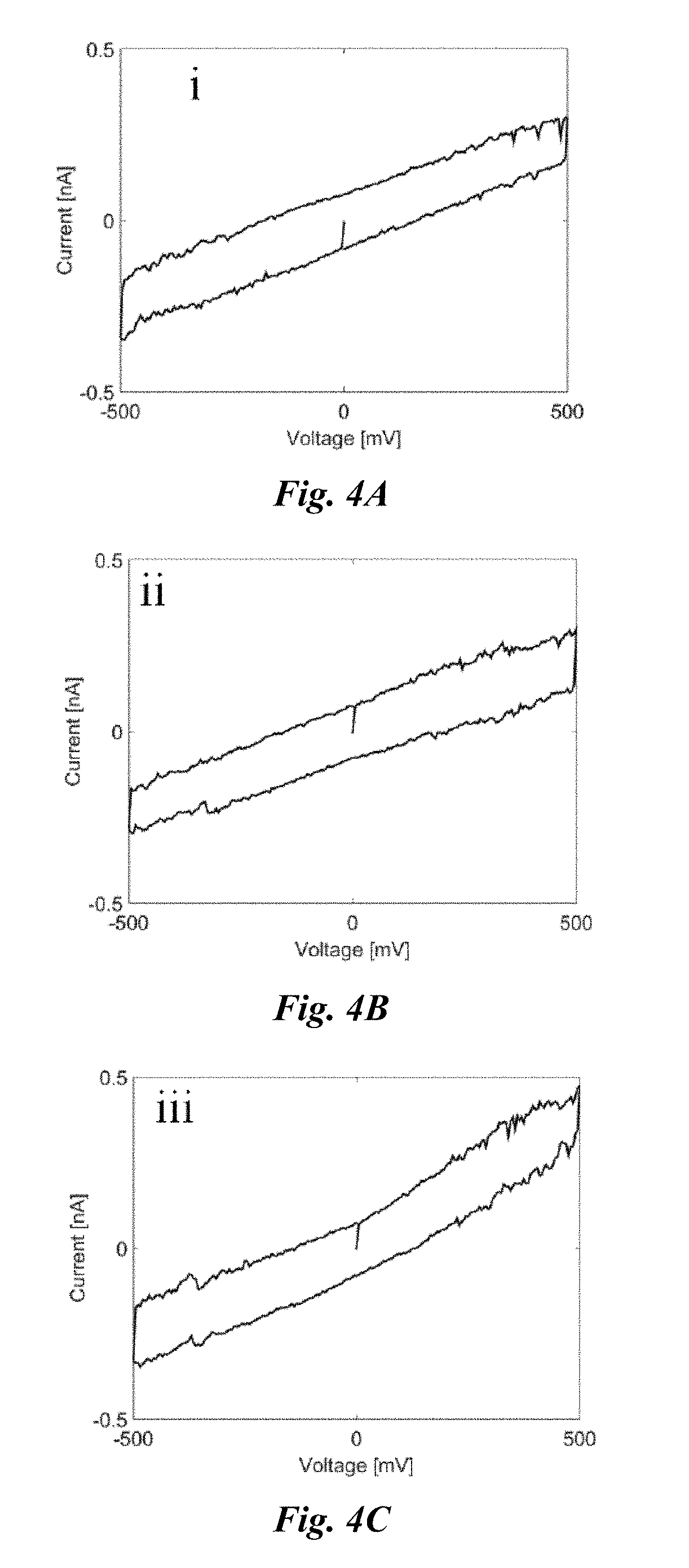
[0029] FIG. 4A shows a typical I-V response of a silicon nitride nanopore drilled by transmission electron microscope (TEM) in 10 mM KCl, PB buffered solution with pH=6.5, at which a rectified ion current can be perceived. The Current-Voltage (I-V) response is an ionic current change with voltage across the membrane.
[0030] FIG. 4B shows a typical I-V response of a silicon nitride nanopore drilled by TEM in 10 mM KCl, PB buffered solution with pH=7.5, at which a rectified ion current can be perceived.
[0031] FIG. 4C shows a typical I-V response of a silicon nitride nanopore drilled by TEM in 10 mM KCl, PB buffered solution with pH=8.5, at which a rectified ion current can be perceived.
[0032] FIG. 5A shows a TEM image of the solid-state nanopore in the silicon nitride membrane for measurement of GAGs.
[0033] FIG. 5B shows a work flow for a multiple run experiment measuring the GAGs translocation through nanopores, which was carried out in a phosphate buffer, pH 7.4.
[0034] FIG. 5C shows typical ionic current traces for 0.4 M KCl, HP.sub.dp20, and CS.sub.dp20 samples and their current spike rates, recorded with a voltage bias of 500 mV.
[0035] FIG. 5D shows histograms of dwell times with their Lognormal fitting curves for HP.sub.dp20 and CS.sub.dp20 at different runs.
[0036] FIG. 5E shows Histograms of blockade ratios with their Gaussian fitting curves for HP.sub.dp20 and CS.sub.dp20 at different runs.
[0037] FIG. 6 shows feature extraction in three domains.
[0038] FIG. 7A shows SVM (support vector machine) determination of CS.sub.dp20 and HP.sub.dp20 compositions of simulated test mixtures. The simulated results are randomly sampled with a certain CS20 ratio from data pool, and tested SVM to compare the result ratio with respect to the desired ratio from two runs with the same nanopore.
[0039] FIG. 7B shows percentages of CS.sub.dp20 determined by nanopore/SVM method against its compositions in the mixture samples as determined from experimental data with several different nanopores.
[0040] FIG. 8A shows TEM image of the nanopore used in the measurement.
[0041] FIG. 8B shows typical ionic current traces of HP.sub.dp20, and CS.sub.dp20, enoxaparin, and UFH recorded under a voltage bias of 500 mV in 0.4 M KCl in phosphate buffer, pH 7.4.
[0042] FIG. 8C shows scatter-plots of dwell time vs current blockade ratio of HP.sub.dp20, and CS.sub.dp20, enoxaparin, and UFH, accompanied with their respective marginal histograms.
[0043] FIG. 9A shows a plot of spike frequency, event rates to the concentrations of HP.sub.dp20 from individual nanopores.
[0044] FIG. 9B shows a plot of averaged frequency event rates to the concentrations of HP.sub.dp20 with their fitting lines. For the linear function, y=log (event rate) and x=log conc.
DEFINITIONS
[0045] "Glycosaminoglycans" (GAGs) or mucopolysaccharides are long unbranched polysaccharides consisting of a repeating disaccharide unit. The repeating unit (except for keratan) consists of an amino sugar (N-acetylglucosamine or N-acetylgalactosamine) along with a uronic sugar (glucuronic acid or iduronic acid) or galactose. Glycosaminoglycans are highly polar and attract water.
[0046] A "calibration sample" is a reference sample, for analysis of known identity and concentration.
[0047] A "nanopore" is an orifice with nanometer diameter and depth in a solid material. The nanopore shape may be irregular and change according to conditions and use, or the nanopore may be fixed in dimensions and may be a regular shape such as circular. One or more nanopores may be assembled in a device to measure electrical signals such as current and voltage.
[0048] "Machine learning" is a statistical technique to iteratively refine and improve models by which raw data can be classified and used to make predictions on data.
[0049] A "Support Vector Machine" or "SVM" refers to a supervised learning model to separate different classes in a hyperdimensional space and is a type of machine learning algorithm, used here as a tool of analyzing data from single molecule detection.
DETAILED DESCRIPTION OF EXEMPLARY EMBODIMENTS
[0050] The invention provides a nanopore and SVM (support vector machine) method to identify, quantify, and characterize heparins and chondroitin sulfate, which represent a class of polysaccharides that pose great challenges to current analytical techniques for their separation and identification due to their varied compositions, charges, and polydispersity. Chondroitin sulfate is a sulfated glycosaminoglycan (GAG) composed of a chain of alternating sugars (N-acetylgalactosamine and glucuronic acid) and is usually found attached to proteins as part of a proteoglycan. A chondroitin chain can have over 100 individual sugars, each of which can be sulfated in variable positions and quantities. Chondroitin sulfate is an important structural component of cartilage.
[0051] The solid-state nanopore is one of the simplest single molecule sensor and SVM is a machine learning algorithm. By combining these two together, heparins and chondroitin sulfate can be identified with high accuracy (>90%) and quantified with high accuracy. Chondroitin sulfate can be identified in a mixture with the heparin to a level as low as 0.8% (w/w). The data indicates that the nanopore/SVM method has potential to identify an impurity present at as low as about 0.5 to 0.05% (molar ratio). In addition, data shows that the nanopore has a limit of detection about 1.0 nanomolar (nM) and 5 decades of magnitude in dynamic range. Also, the nanopore/SVM technique distinguished between unfractionated heparin (UFH) and enoxaparin with an accuracy of about 94% on average. Using a reference sample to calibrate nanopores, heparin is quantified using different nanopores with reasonable accuracy, achieving nanomolar sensitivity and a 5-Log dynamic range, demonstrating that the nanopore/SVM technique can be used to monitor heparins and identify GAGs. These results show that the nanopore technique powered by machine learning can be a simple and cheap tool for monitoring heparins and other glycosaminoglycans (GAGs) from lot to lot with reference to standard samples that are fully characterized by NMR, mass spectrometry, and other analytic methods.
[0052] The present invention employs a silicon nitride nanopore for differentiation between GAGs, such as two sulfated GAGs; heparin and oversulfated chondroitin sulfate (OSCS).
[0053] Both heparin and OSCS in a mixture can be qualitatively identified either by current blockade magnitudes or blockade durations despite considerable overlaps of these parameter distributions in a 2D scatter plot. Nano-electronic technologies are useful for the identification and sequencing of carbohydrates. Solid-state nanopores can be used to distinguish heparins from chondroitin sulfate on a single molecule basis with the aid of machine learning, and the frequency of translocation signals can be used for heparin quantitation over a wide dynamic range. As illustrated in FIG. 1A, when a negatively charged GAG molecule translocates through a silicon nitride nanopore under a voltage bias, it can cause a transient blockade of ionic current, generating a spike; an event that carries information on the structure and physical properties of the GAG molecule as it interacts with the nanopore. FIG. 1B shows current traces of monodispersed heparin (HP.sub.dp20) and chondroitin sulfate (CS.sub.dp20) fragments generated by nanopore measurements. Herein, HP.sub.dp20 denotes a heparin fragment that is composed of 20 sugar units (dp: degree of polymerization), and CS.sub.dp20 chondroitin sulfate fragment that is comprised of 10 disaccharide units of .beta.-D-glucuronic acid-(1.fwdarw.3)-.beta.-N-acetylgalactosamine-4-sulfate (1.fwdarw.4) (Lamari, F. N. & Karamanos, N. K. in Chondroitin Sulfate: structure, role and pharmacological activity, Vol. 53. (eds. J. T. August, D. Granner & F. Murad) 33-48 (2006) Elsevier Inc.). Each individual signal was characterized by its blockade ratio (of the spike amplitude to baseline ionic-current) and dwell time (width of the spike). Each of these individual parameters exhibited similar distributions between HP.sub.dp20 and CS.sub.dp20. As shown in FIGS. 1C and 1D, the probability of separating HP.sub.dp20 from CS.sub.dp20 by their dwell times is about 54%, and the probability by their blockade ratios is about 61% (slightly better than a random pick that is 50%). When these two parameters are plotted together as the probability density for the simultaneous appearance of a pair of values in a given spike, it improves the separation to >66%. Higher accuracy may be achieved in a high dimensional space to classify the nanopore data with the use of machine learning for analysis of the nanopore data, engaging Support Vector Machines (SVMs). SVM is a supervised learning model to separate different classes in a hyperdimensional space and is used here as a tool of analyzing data from single molecule detection. SVM is employed here to analyze solid-state nanopore translocation data of GAG molecules.
[0054] Identification of heparins and related GAGs: Heparin, a member of a group of sulfated glycosaminoglycans (GAGs) has the repeating structure:
##STR00003##
[0055] Heparin (CAS Reg. No. 9005-49-6) has a molecular weight of about 12,000-15,000 and is a naturally occurring anticoagulant produced by basophils and mast cells. In therapeutic doses, it acts as an anticoagulant, preventing the formation of clots and extension of existing clots within the blood.
[0056] Heparins were identified using a nanopore device (FIG. 1A). The ionic current blockages of both HP.sub.dp20 and CS.sub.dp20 were measured in a nanopore using the device shown in FIG. 1A, generating translocation current signals. When the GAG molecules translocate through the silicon nitride nanopore, they transiently block the ionic current and produce spikes that can be recorded as a signal train with time. FIG. 1B shows spectra of current traces generating by translocation of a monodisperse heparin (HP) fragment designated as HP.sub.dp20, which is composed of 20 sugar units (dp: degree of polymerization), and a GAG counterpart, chondroitin sulfate (CS.sub.dp20) that is composed of 10 disaccharide units of sulfated .beta.-D-glucuronic acid-(1.fwdarw.3)-.beta.-N-acetylgalactosamine-(1.fwdarw.4) (Lamari, F. N.; Karamanos, N. K. Structure of Chondroitin Sulfate. In Chondroitin Sulfate: Structure, Role and Pharmacological Activity, August, J. T.; Granner, D.; Murad, F., Eds. Elsevier Inc.: 2006; Vol. 53, pp 33-48). Although these two GAGs are composed of monodisperse oligosaccharides, they contain different sulfation patterns, respectively.
[0057] Nanopore/SVM Identification of HP.sub.dp20 and CS.sub.dp20.
[0058] Monodisperse GAG samples HP.sub.dp20 and CS.sub.dp20 were characterized by size exclusion (FIG. 2A) and anion-exchange HPLC (FIG. 2B). Both have similar molecular weights, but HP.sub.dp20 is more negatively charged than CS.sub.dp20. Density Functional Theory (DFT) modeling shows that the most common disaccharide units in heparin and CS have distinct structural features, but both of them are highly negatively charged. DFT is a computational quantum mechanical modelling method used in physics, chemistry and materials science to investigate the electronic structure (principally the ground state) of many-body systems, in particular atoms, molecules, and the condensed phases. These differences in their electrical properties enable the nanopore to distinguish between HP.sub.dp20 and CS.sub.dp20. The solid-state nanopores were fabricated in a silicon nitride membrane by drilling with a transmission electron microscope (TEM), most likely generating an hourglass-shaped geometry (Kim, M. J., et al (2007) Nanotechnology 18:205302). Given that the surface of silicon nitride is zwitterionic with an isoelectric point around pH 7, these nanopores should have their surface charges close to neutral in a buffer, pH=about 7.4, at which the translocation experiments were carried out. Around the pH value, rectified currents were not clearly observed (FIGS. 4A-C). By a reversing bias experiment, FIG. 3B shows that HP.sub.dp20 was able to translocate through a solid state nanopore. It may be an indicator of a neutral surface because the rectification requires an asymmetric electrical double layer within the nanopore. In a 0.4 M KCl electrolyte solution buffered with 1.0 mM phosphate buffer, pH 7.4, the nanopore generated a 2 nA ionic current with a stable baseline (FIG. 3A). Switching the bias from the positive to negative changed the current polarity and slightly increased the width of the baseline. When a HP.sub.dp20 solution was injected with a 1.0 .mu.M final concentration of 1.0 .mu.M in the cis-chamber of the nanopore where the electrode was grounded, frequent current blockade events (spikes) were observed under a positive bias, but no blockade signals under a negative bias (FIG. 3B). A 600 mV bias was applied for two hours and the ionic current was measured again. Blockage signals were observed from both positive and negative biases (FIG. 3C). These results can best be explained by HP.sub.dp20 molecules being translocated from the cis to trans chamber through the nanopore. In general, a thinner nanopore should give better resolution, but is more fragile than a thicker one. After comparing the translocation in nanopores with different thickness (15, 30, and 50 nm), a 30 nm thick silicon nitride membrane was selected for its easy of handling and less probability of multi-molecule blockade (FIGS. 3A-C). Also by a reverse bias experiment, it was confirmed that HP.sub.dp20 translocated through a solid-state nanopore of about 3.0 nm in diameter (FIGS. 3A-C). Following this benchmark work, serial measurements on HP.sub.dp20 and CS.sub.dp20 with a newly fabricated silicon nitride nanopore. FIG. 5A shows the transmission electron microscope (TEM) image of a nanopore.
[0059] FIG. 5B shows a work flow for the translocation measurements of analytes. It begins with running a PBS buffer, followed by injecting first sulfated GAG (here it is HP.sub.dp20), second sulfated GAG (here it is CS.sub.dp20), and then rinse the nanopore to finish the first run (Run-1). The process is repeated in the second run (Run-2) either with the same samples or with samples to be tested. In general, the first run samples can be standard samples and second ones can be those to be analyzed. As illustrated in FIG. 5B, the two GAG samples were sequentially measured in Run-1 and Run-2. Note that there was a process of rinsing the nanopore and stabilizing (or recovering) the baseline prior to measuring each of the samples. FIG. 5C displays traces of ionic currents recorded from each discrete measurements of 0.4 M KCl, HP.sub.dp20, and CS.sub.dp20, where each spike may represent a single molecule translocating or bumping event, a "translocation current signal". At first glance, HP.sub.dp20 shows higher event rates than CS.sub.dp20, and the event rates of CS.sub.dp20 varied more significantly than those of HP.sub.dp20 from run to run. Nanopore data was analyzed by dwell times and blockade ratios of individual spikes, and plotted in histograms shown in FIGS. 5D and 5E, respectively. The distributions of dwell times were best fit to the Lognormal function, whereas those for blockade ratios were best fit to the Gaussian function, from which statistical values of these parameters were derived for both HP.sub.dp20 and CS.sub.dp20 and summarized in Table 1. These parameters are only marginally different from Run-1 to Run-2 for both HP.sub.dp20 and CS.sub.dp20, indicating that the nanopore measurement is reasonably reproducible. Statistically, each parameter distribution shows significant overlap between HP.sub.dp20 and CS.sub.dp20 (see FIGS. 5D and 5E). These primary parameters are not sufficient for discriminating among monodisperse GAG samples unambiguously.
TABLE-US-00001 TABLE 1 Statistical parameters derived from curve fitting of raw data in FIGS. 5D and 5E HP.sub.dp20 CS.sub.dp20 Dwell Time Blockade Dwell Time Blockade (ms) Ratio (ms) Ratio Median Mean Mean .sigma. Median Mean Mean .sigma. Run-1 0.083 0.092 0.120 0.027 0.080 0.092 0.105 0.019 Run-2 0.087 0.098 0.118 0.027 0.073 0.081 0.111 0.028 Note: (1) all adj. R.sup.2 >95%; (2) all fitting errors for median <.+-.1.0% and for mean <.+-.1.0%; (3) all fitting errors for Peak <.+-.0.1% and for Width <.+-.0.2%. ms = milliseconds
[0060] Machine learning, particularly SVM, was used to analyze the translocation current signals of the nanopore data. SVM is a method that requires many independent parameters (or features) to classify data in a hyperdimensional space. A plethora of features were extracted by Fourier transform (FFT) and cepstrum transform of the nanopore data recorded in the time domain to index individual spikes (FIG. 6). A cepstrum is the result of taking the Inverse Fourier transform (IFT) of the logarithm of the estimated spectrum of a signal. For the machine learning, 50% of the nanopore data was randomly taken either from Run-1 or Run-2 to train SVM until it could successfully assign each of the spikes in the training data to its corresponding GAG analyte with 100% accuracy (Table 2). SVM could be trained with different combinations of features, as a trained machine learning algorithm, to achieve the same 100% accuracy, i.e. many different SVMs can be created using the same data set (Example 3, Table 11). To score, these trained SVMs were engaged to call the remaining 50% of the randomly selected nanopore data by scaling a perfect calling accuracy to 100%. As shown in Table 2, SVM-2 has the highest rating of 92.7 among those trained with the Run-1 data, and SVM-4 has the highest score of 95.1 among those trained with the Run-2 data on average. SVM-2 was used to call the Run-2 data, which identified HP.sub.dp20 and CS.sub.dp20 with an accuracy of 94.2% and 95.1%, respectively. Similarly, SVM-4 called HP.sub.dp20 and CS.sub.dp20 in the Run-1 data with an accuracy of 93.7% and 91.2%, respectively. In either instance, SVM called these two GAGs with high accuracy. It should be noted: (1) the accuracy is related to SVM calling single spikes. Assuming the errors occur randomly, one may expect that it can be further improved by multiple nanopore measurements; (2) the nanopore data may be a sum of molecular bumping and translocating events. The above results suggest that both bumping and translocating data can be used by the SVM to identify the GAG molecules.
TABLE-US-00002 TABLE 2 Accuracy of SVM calling individual spikes SVM Calling SVM Training Remaining Training No. Training 50% data Untrained data data set Analyte Features accuracy HP.sub.dp20 CS.sub.dp20 HP.sub.dp20 CS.sub.dp20 SVM-2 50% of HP.sub.dp20 11 100 93.2 7.9 Run-2 94.2 4.9 Run-1 CS.sub.dp20 6.8 92.1 5.8 95.1 SVM-4 50% of HP.sub.dp20 11 100 96.2 6.0 Run-1 93.7 8.8 Run-2 CS.sub.dp20 3.8 94.0 6.3 91.2
[0061] Detection of CS.sub.dp20 in a binary mixture. The nanopore/SVM method was tested for its potential use in the detection of impurities in a heparin product. CS.sub.dp20 was mixed with HP.sub.dp20 in a molar percentage of 1%, 5%, 10%, 20%, and 50%, respectively. The nanopore measurement was carried out in the same way as described above, following a sequence of CS.sub.dp20, HP.sub.dp20, and the mixture. Here, the pure CS.sub.dp20 and HP.sub.dp20 samples were used as standards to produce the reference data for training SVM. The nanopore was easily blocked by these mixtures presumably during the translocation process. However, the measurements were also conducted using multiple nanopores. As shown in Table 3, six nanopores were used in this study, and each mixture was measured at least twice either by the same nanopore or different nanopores.
TABLE-US-00003 TABLE 3 CS.sub.dp20 molar percentages in mixtures determined by the nanopore/SVM method Molar percentage of CS.sub.dp20 in HP.sub.dp20 SVM 1% 5% 10% 20% 50% Nanopore score Percentage (%) of CS.sub.dp20 determined by SVM calling Pore-1 98.3 46.1 Pore-1.sup..alpha. 100 57.2 Pore-2 93.3 1.4 11.1 Pore-3 94.0 3.0 7.4 Pore-4 84.1 23.2 Pore-5 83.3 0.5 3.9 Pore-6 80.8 9.3 21.9 Average .+-. SEM.sup.b 1.6 .+-. 0.7 5.7 .+-. 1.8 10.2 .+-. 0.9 22.6 .+-. 51.7 .+-. CV (%).sup.c 0.7 5.6 Error rate (%).sup.d 77.5 43.8 12.5 4.1 15.2 60.0 14.0 2.0 13.0 3.4 .sup.aa repeat of the measurement in Pore-1; .sup.bSEM: standard error of mean; .sup.cCV: coefficient of variation; .sup.dError rate = <averaged called percentage - molar percentage in sample>/molar percentage in sample.
[0062] Following the nanopore measurement, SVM with data from the reference samples was trained in the same manner as described above and engaged the SVMs to call HP.sub.dp20 and CS.sub.dp20 in the mixtures from their nanopore data (Table 4). Table 4 lists the percentages of CS.sub.dp20 in the different mixtures determined by the best-scored SVM. Although the measured percentage of CS.sub.dp20 varies more or less from nanopore to nanopore, which may be attributed to the variations in the geometry of nanopores, the average is close to the correct percentage existing in the mixture. A plot of the average called percentages against molar percent of CS.sub.dp20 in the mixtures fits a linear function (FIG. 7B). With its intercept fixed at the origin, the fit gives the trendline a slope of about 1.1, slightly higher than 1.0 which is the best-case scenario, and which may result in an overestimate of CS.sub.dp20 by 10%. Overall, the variations among different pores decrease with increases of CS.sub.dp20 percentage in the mixture, as do the SVM calling error rates (based on CV values and error rates in Table 3). This study demonstrates the nanopore/SVM method can identify CS.sub.dp20 in a mixture down to about 1% in molar percentage, equal to a weight percentage of 0.8% (w/w). This sensitivity is comparable to 500 MHz NMR, which has a limit of detection of 0.1% w/w for oversulfated chondroitin sulfate (OSCS)..sup.39 However, NMR requires milligrams of sample/0.7 mL solvent for the measurement so that the OSCS ought to be at least at a microgram level in the sample. For the nanopore measurement, 0.1 mL of solution was used with the mixture containing a total GAG concentration of 100 nM. To measure the 1% mixture, only 0.4 ng of CS.sub.dp20 was needed for the nanopore detection.
TABLE-US-00004 TABLE 4 SVM scores of repeat measurements with same nanopore Molar percentage of CSdp20 in HP.sub.dp20 1% 5% 10% 20% 50% Total Events No. SVM Percentage (%) of CSdp20 determined by SVM Nanopore HP.sub.dp20 CS.sub.dp20 Mixtures Features score calling Pore-1 399 914 631 7 98.3 46.1 10 97.4 45.1 11 98.0 44.8 pore-1.sup.a 278 195 957 10 100 57.2 11 100 62.3 12 99.6 65.3 Pore-2 853 1012 1011/1933 6 91.9 1.2 9.9 6 92.0 0.3 12.4 11 93.3 1.4 11.1 Pore-3 219 845 2697/95 4 90.6 1.7 6.3 4 90.6 2.0 8.7 14 94.0 3.0 7.4 Pore-4 1731 1931 2180 9 82.5 22.8 14 84.0 22.8 15 84.1 23.2 Pore-5 9663 1265 22029/9177 20 79.4 0.2 6.0 23 83.3 0.5 3.9 26 81.8 0.5 4.5 Pore-6 3317 1844 2560/2205 8 80.2 8.9 20.3 10 80.8 9.3 21.9 12 80.4 7.4 19.3
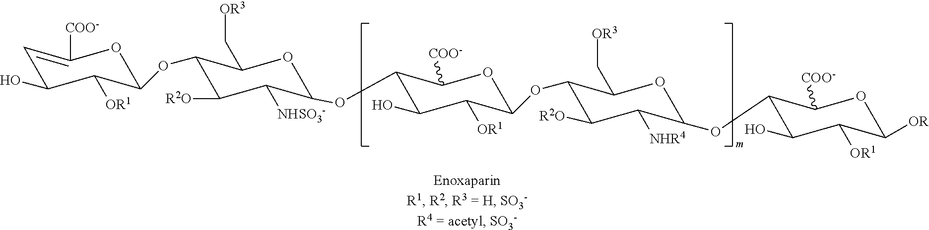
[0063] Identification of unfractionated heparin and enoxaparin. To explore its potential application in pharmaceutical production, the nanopore/SVM method was tested on samples with clinical uses, e.g. unfractionated heparin (UFH) and a LMWH (low molecular weight heparin) drug enoxaparin (enoxaparin sodium: CAS Reg. No. 9005-49-6, trade names: Lovenox.RTM., Clexane.RTM., Xaparin.RTM.). UFH and LMWH drugs are widely used in the prevention and treatment of thromboembolic disorders (Cosmi, B. et al, Thromb. Res. (2012) 129:388-91; Lee, S. et al, Nat. Biotechnol. (2013) 31:220-6). Enoxaparin, with an average MW of about 4500, is a product of depolymerizing the UFH, so called low molecular weight heparins (LMWH), a mixture of polydisperse oligosaccharides each containing an unsaturated urinate residue at its non-reducing end and an amino sugar or a 1,6-anhydro amino sugar at its reducing end. Nonetheless, the enoxaparin still remains about 20% of antithrombin-binding fractions of UFH (Mourier, P. A. et al, J. Pharm. Biomed. Anal. 2015, 115:431-42). Besides being shorter than UFH, enoxaparin is also polydisperse and contains an unsaturated uronate residue at its non-reducing end as well as an amino sugar or a 1,6-anhydro amino sugar at its reducing end, having the structure:
##STR00004##
[0064] Serial measurements of HP.sub.dp20, CS.sub.dp20, enoxaparin, and UFH were conducted at 1.0 .mu.M concentrations using a newly drilled nanopore of about 3 nm in diameter (FIG. 8A). Between the measurements, there was a process of rinsing and baseline recovery. FIG. 8B displays the typical current traces of these GAG products recorded by the nanopore and their event rates which follow an order of UFH>HP.sub.dp20>enoxaparin>CS.sub.dp20. First, the current spikes of each product were characterized by their dwell times and blockade ratios, which were then placed in a 2D scatter plot (FIG. 8C). The most noticeable feature is that UFH displays a two-peaked distribution in its blockade ratios, one of which is located at the low end between 0.1 to 0.2, the same as the other GAGs, and the other located between 0.6 to 0.8, which can be attributed to a significant portion of high molecular weight fraction existing in UFH. Also, these GAG products have their dwell times in a range of 60 to 90 microseconds (.mu.s) on average (Table 10). Since the data was recorded at a sampling rate of 500 kHz with 100 kHz low pass frequency bandwidth, the differences among those dwell times may not be significant.
TABLE-US-00005 TABLE 5 Dwell Times derived from curve fitting to the Lognormal function HPdp20 CSdp20 Enoxaparin UFH Median (ms) 0.063 0.074 0.064 0.061 Mean (ms) 0.069 0.091 0.071 0.083 Adj. R.sup.2 0.98 0.99 0.97 0.98
[0065] To identify these GAGs, 50% of the data was randomly selected from each of collected data sets to train the SVM with up to 88 available signal features and then applied the trained SVM to classify the rest of 50% remaining data. The effectiveness of SVM for the GAG identification is quickly determined without laborious multiple runs. The four products can be distinguished in pairs by SVM. All of SVMs were trained to be capable of identifying individual spikes in the training data with 100% accuracy, as a trained machine learning algorithm. As shown in Table 5, both UFH and CS.sub.dp20 were called with an accuracy of 94.6% and 91.0%, respectively, 92.5% on average (Entry 1); UFH and enoxaparin (designated as Enox) with an accuracy of about 96% and 93%, respectively (Entry 2). However, UFH and HP.sub.dp20 were distinguished with a lower accuracy of about 85% on average (Entry 3). For calling Enox, the SVM distinguished between Enox and HP.sub.dp20 (Entry 5) marginally better than between UFH and HP.sub.dp20. The SVM distinguished between Enox and CS.sub.dp20 with an averaged accuracy of about 73% (Entry 4), significantly lower than it did between UFH and CS.sub.dp20 which is consistent with the scatter plots in FIG. 8C, where the data points of CS.sub.dp20 overlaps with those of enoxaparin more than those of UFH. SVM distinguished between HP.sub.dp20 and CS.sub.dp20 (Entry 6) better than between Enox and CS.sub.dp20 (Entry 4), even though HP.sub.dp20 has a molecular weight distribution overlapped with CS.sub.dp20 more than enoxaparin does with CS.sub.dp20 (FIG. 2A). Thus, the result may be better explained based on their Anion-Exchange (SAX)-HPLC chromatograms (FIG. 2B), where HP.sub.dp20 has charged fragments overlapped with CS.sub.dp20'S less than enoxaparin does. The nanopore shown in FIG. 5A had a higher accuracy for distinguishing between HP.sub.dp20 and CS.sub.dp20 than the one in FIG. 8A did. From their TEM images, these two nanopores had different shapes and diameters, which should contribute to the reduced accuracy. Furthermore, SVM was tested for calling all of the four GAG products from a pool of the nanopore data. The SVM called UFH with an accuracy of about 80% and the rest with accuracy around about 65% (Entry 7). These calling accuracies are statistically significant because the probability of a random pick would only be 25%. The better calling accuracy for UHF could be explained by the fact that UHF contains a portion of blockade currents well separated from those of the rest of the GAGs, which are overlapped with one another (FIG. 8C). Nonetheless, the low calling accuracy indicates that the data from a single nanopore would not be sufficient for SVM to call multiple GAGs all at once.
TABLE-US-00006 TABLE 6 Accuracy of SVM calling heparins and CS.sub.dp20 Training Accuracy Identification accuracy (%).sup.1 Entry Entity (%) UFH CS.sub.dp20 Enox. HP.sub.dp20 Average 1 UFH vs 100 94.6 .+-. 1.2 91.0 .+-. 1.5 92.5 .+-. 1.0 CS.sub.dp20 2 UFH vs 100 95.9 .+-. 0.9 92.9 .+-. 0.9 94.4 .+-. 0.6 Enox 3 UFH vs 100 87.2 .+-. 1.6 82.1 .+-. 1.4 84.7 .+-. 1.1 HP.sub.dp20 4 Enox vs 100 73.8 .+-. 2.7 72.1 .+-. 1.7 73.0 .+-. 1.6 CS.sub.dp20 5 Enox vs 100 88.4 .+-. 2.3 86.4 .+-. 1.3 87.4 .+-. 1.3 HP.sub.dp20 6 HP.sub.dp20 vs 100 88.7 .+-. 1.8 83.3 .+-. 1.4 86.0 .+-. 1.1 CS.sub.dp20 7 Pool of 100 80.6 .+-. 1.6 65.1 .+-. 2.6 65.2 .+-. 3.3 64.8 .+-. 3.3 68.9 .+-. 1.4 Four .sup.1each value is an average of three calls by the SVMs trained from three randomly selected subsets of data.
[0066] Quantification of HP.sub.dp20.
[0067] The use of solid-state nanopores was demonstrated for quantitation of sulfated GAGs. In the nanopore measurement, the event rate changes with the concentration of an analyte. Thus, the determination of concentrations becomes counting of spikes. Event rates linearly increased with concentrations of heparin in a range of 0.25 to 1.25 .mu.M (a five-fold change). The HP.sub.dp20 concentration was measured ranging from 1.0 nM to 100 .mu.M using multiple nanopores to build a calibration curve with calibration samples. For the measurement, each concentration was repeated at least once in the same or a different nanopore. From the nanopore data was extracted all of the ionic current signals above a threshold as conducted for the SVM analysis, defining an event rate as spikes/s (Table 7). The event rate varied from nanopore to nanopore for the same concentration. That may be attributed to different diameters and shapes among these nanopores even though they were fabricated under the same TEM conditions.
TABLE-US-00007 TABLE 7 Translocation Frequencies of HPdp20 through nanopores (spikes/sec) Nanopore Sample dilution [.mu.M] pore d [nm] 0.001 0.01 0.05 0.1 0.5 1 3.3 3.078 .+-. 0.529 3.259 .+-. 0.177 2 2.0 0.143 .+-. 0.014 0.199 .+-. 0.018 0.270 .+-. 0.057 0.358 .+-. 0.052 2* 2.0 0.147 .+-. 0.016 0.399 .+-. 0.041 3 2.5 0.760 .+-. 0.067 4 2.5 0.101 .+-. 0.011 0.157 .+-. 0.015 5 2.6 0.088 .+-. 0.012 0.536 .+-. 0.158 0.859 .+-. 0.147 1.204 .+-. 0.109 6 3.2 0.272 .+-. 0.022 0.335 .+-. 0.047 7 2.7 0.120 .+-. 0.017 0.138 .+-. 0.016 0.441 .+-. 0.018 8 3.6 0.597 .+-. 0.053 1.663 .+-. 0.510 Nanopore Sample dilution [.mu.M] pore d [nm] 1 5 10 100 1 3.3 5.716 .+-. 0.299 2 2.0 3.477 .+-. 0.211 2* 2.0 3 2.5 2.319 .+-. 0.656 3.503 .+-. 1.404 4 2.5 6.891 .+-. 0.631 5 2.6 9.530 .+-. 0.947 6 3.2 1.189 .+-. 0.207 2.098 .+-. 1.260 7 2.7 1.082 .+-. 0.080 9.573 .+-. 0.762 8 3.6 4.373 .+-. 0.507
[0068] In order to compare the event rates between nanopores, all the event rates measured were normalized with the same nanopore by referencing the one at 0.1 .mu.M as 1.0 (Table 8).
TABLE-US-00008 TABLE 8 Normalized frequencies (referenced to those from 0.1 .mu.M sample as 1) Nanopore Sample dilution micromolar (.mu.M) pore d [nm] 0.001 0.01 0.05 0.1 0.5 1 3.3 1.000 .+-. 0.172 1.058 .+-. 0.057 2 2.0 0.400 .+-. 0.041 0.554 .+-. 0.050 0.752 .+-. 0.160 1.000 .+-. 0.146 2* 2.0 0.368 .+-. 0.042 1.000 .+-. 0.103 3 2.5 1.000 .+-. 0.088 4 2.5 0.648 .+-. 0.070 1.000 .+-. 0.099 5 2.6 0.102 .+-. 0.014 0.623 .+-. 0.184 1.000 .+-. 0.171 1.400 .+-. 0.127 6 3.2 0.812 .+-. 0.067 1.000 .+-. 0.141 7 2.7 0.274 .+-. 0.039 0.314 .+-. 0.036 1.000 .+-. 0.041 8 3.6 0.359 .+-. 0.032 1.000 .+-. 0.306 Ave. 0.286 .+-. 0.133 0.469 .+-. 0.158 0.729 .+-. 0.096 1.000 .+-. 0.000 1.229 .+-. 0.241 Nanopore Sample dilution micromolar (.mu.M) pore d [nm] 1 5 10 100 1 3.3 1.856 .+-. 0.097 2 2.0 9.688 .+-. 0.589 2* 2.0 3 2.5 3.051 .+-. 0.863 4.609 .+-. 1.847 4 2.5 43.894 .+-. 4.024 5 2.6 11.085 .+-. 1.102 6 3.2 3.551 .+-. 0.619 6.264 .+-. 3.762 7 2.7 2.453 .+-. 0.182 21.693 8 3.6 2.629 .+-. 0.305 Ave. 2.708 .+-. 0.637 5.436 .+-. 1.170 10.386 .+-. 0.987 32.793 .+-. 15.69
[0069] The normalized data plotted on a log-log scale (FIG. 9A) appear to increase exponentially with concentrations of HP.sub.dp20. However, their averages in the low and high concentration regions can separately be fit into two different linear functions of the logarithmic variables, as displayed in FIG. 9B which is consistent with changes of event rates with the DNA concentrations. The data also indicates that the event rates change more rapidly in the micromolar (.mu.M) region than in the nanomolar (nM) region. It is estimated that the nanopore measurement for the detection of HP.sub.dp20 can reach a nanomolar (nM) level with a 5-Log dynamic range, a standard curve for the determination of HP.sub.dp20 concentrations.
[0070] Using two newly fabricated nanopores, the standard curve was tested for the HP.sub.dp20 samples. In the same way as shown in FIGS. 9A and 9B, the 0.1 .mu.M HP.sub.dp20 sample was used as a control and its event rates in the nanopores were referenced as 1.0 (Table 7).
TABLE-US-00009 TABLE 9 Raw and normalized event rate of the pores used in Table 10 Pore Concentration [.mu.M] Index 0.01 0.05 0.1 1 5 5-1 Raw Event Rate 0.676 1.002 1.573 2.396 9.714 Normalized Event Rate 0.430 0.637 1.000 1.523 6.175 Determined conc. 0.008 0.03 -- 0.6 4.7 5-2 Raw Event Rate 0.796 -- 1.563 3.854 -- Normalized Event Rate 0.509 -- 1.000 2.466 -- Determined conc. 0.013 -- -- 1.2 --
[0071] As shown in Table 10, four HP.sub.dp20 samples were measured for their event rates with a nanopore (designated as Pore 9), from which their concentrations were derived by applying either of the two functions in FIG. 9B, and then repeated the measurement with two of the samples using the second nanopore (designated as Pore 10). The results show that each concentration determined by the single nanopores considerably deviates from its actual value in the tested sample and also varies from nanopore to nanopore. For example, the 0.01 LM sample was determined as 0.008 LM by Pore 9 and 0.013 LM by Pore 10. However, the average of these two measurements is 0.011, only 10% off from the actual concentration. For the 1.0 LM sample, the average of measurements by these two nanopores is 0.9 M, just 10% lower than expected. At the higher 5.0 LM concentration, the concentration determined by a single nanopore measurement deviated from the actual value by 6%, demonstrating that the nanopore can be used to quantify the sulfated GAG samples by introducing a reference sample for the nanopore calibration. Moreover, the multiple-nanopore measurement may achieve a high accuracy when the sample concentration is below micromolar (M) level.
TABLE-US-00010 TABLE 10 Fitting functions for determination of HP.sub.dp20 concentration by nanopores Concentration Measurement Pore Sample conc. (.mu.M) 0.01 0.05 1.0 5.0 9 Event rate* 0.430 0.637 1.523 6.175 (spikes/s) Derived conc. (.mu.M) 0.008 0.025 0.6 4.8 10 Event rate* 0.509 -- 2.466 -- (spikes/s) Derived conc. (.mu.M) 0.013 -- 1.20 -- Average (.mu.M) 0.011 .+-. 0.004 0.90 .+-. 0.42 *normalized event rates and see Table 7 for their raw data.
[0072] A nanopore/SVM method for identification of sulfited GAGs is demonstrated that distinguishes between heparins as well as between heparin and chondroitin sulfate with high accuracies. The nanopore/SVM method was also able to identify CS.sub.dp20 in its mixtures with HP.sub.dp20 at a level down to 0.8% (w/w), comparable to the NM R technique for detection of OSCS. Besides its bulkiness and expensiveness, NMR spectrometers also require more materials for the analysis.
[0073] To address the issue on non-uniformity of nanopore size and geometry, a reference sample (calibration sample) was used for the calibration of nanopores (0.1 .mu.M HP.sub.dp20) which allowed normalization of the data from different nanopores. 1 h was observed HP.sub.dp20 can be quantified with reasonable accuracy by the multiple-nanopore measurement. Nanopore measurement has a nanomolar (nM) limit of detection and five orders of magnitude dynamic range. Thus, such a nanopore device can potentially be used to monitor the heparin level in the human blood since the range of plasma heparin is about 1 to 2.4 mg per liter, equivalent to a range of 67 to 160 nM (assuming an average molecular weight of 15,000 for UFH). An array of nanopores may be produced and used to optimize different machine learning algorithms for the identification of GAGs.
EXAMPLES
Example 1 Fabrication of Nanopores
[0074] Silicon chips (5.times.5 mm) coated with silicon nitride (30 nm thick) were purchased from Norcada Inc. (part number: NX5025X). Following a process of argon plasma cleaning, nanopores were drilled using the electron beam in JEOL 2010FEG and ARM 200F transmission electron microscope (TEM) at 200 keV. The size of the pores was controlled by the electron beam size and exposure time. The nanopores were imaged right after the drilling. The nanopore was drilled in a 30 nm-thick silicon nitride membrane by TEM, which shows a conical shape with a diameter of about 3.2 nm at its narrowest section (FIG. 8A).
Example 2 Preparation of Sample Solutions
[0075] Stock solutions of HP.sub.dp20 and CS.sub.dp20 (Iduron) were prepared respectively by dissolving the sample in H.sub.2O. Their actual concentrations were determined based on the carbazole assays. These two stock solutions of HP.sub.dp20 (10 mM) and CS.sub.dp20 (10 mM) were used to prepare mixtures of HP.sub.dp20 and CS.sub.dp20 with a ratio of 1, 5, 10, 20, and 50% of CS.sub.dp20. The final concentrations of these mixtures were diluted to be 0.5-1 .mu.M with an electrolyte solution of 0.4 M KCl in 1 mM phosphate buffer (pH 7.4). For the dilution study, the 10 mM stock solution of HP.sub.dp20 was diluted to various concentrations in a range of 1 mM to 10 nM and injected into the cis reservoir to make the final concentrations of the analyte 100 .mu.M to 1 nM for the measurement.
Example 3 Nanopore Measurements
[0076] Prior to the measurement, a nanopore chip was cleaned by immersing in a hot piranha acid (piranha etch) solution (H.sub.2O.sub.2:H.sub.2SO.sub.4=1:4) for 20 min, and then rinsed with Milli-Q water (a resistivity of about 18.2 M.OMEGA..times.cm and total organic carbon of less than 5 ppb). Piranha acid solutions are extremely energetic and may result in explosion or skin burns if not handled with extreme caution. After drying with N.sub.2 gas, the nanopore chip was placed in a piranha-cleaned PCTFE cell to form a cis reservoir and sealed with a quick-curing silicone elastomer gasket. The PCTFE cell with a nanopore chip was then assembled with a PTFE base to form a trans reservoir. The electrolyte solution used was 0.4 M KCl in 1 mM phosphate buffer (pH 7.4), which was filtered with a Millipore 0.2 .mu.m filter. Ag/AgCl electrodes, freshly made from Ag wires with bleach, were inserted into both cis and trans reservoirs for ionic current measurement. All of analytes were dissolved in the electrolyte solution for the nanopore analysis.
[0077] For the measurement, both cis and trans reservoir were filled with the electrolyte solution, and the nanopore was soaked for about 1 to 2 hours, followed by applying a high voltage (about 1 V) between two reservoirs for about 5 to 10 minutes to obtain a steady baseline current and no electrical spikes, an indicator of achieving an open and wet nanopore. Then, an analyte solution (about 10 .mu.l) was injected into the cis reservoir with a final concentration of about 1 .mu.M. A translocation bias was applied to the Ag/AgCl electrode in the trans reservoir, while the electrode in the cis reservoir was kept grounded to avoid adsorption of analyte molecules to the reference electrode. After recording the ionic current, the cis reservoir was drained and rinsed with the electrolyte solution. Another baseline was recorded to ensure no contaminations left in cis reservoir before a new analyte solution was injected.
TABLE-US-00011 TABLE 11 SVM scores of repeat measurements with same nanopore SVM Training Training SVM score on SVM score on Data trained data set untrained data set (Prediction No. Training Analyte HP.sub.dp20 CS.sub.dp20 HP.sub.dp20 CS.sub.dp20 SVM Index Data) Features Score (Events) (609) (361) (1640) (1271) SVM-1 Run-1 11 100 HP.sub.dp20 92.6 9.4 93.4 6.5 (Run-2) (610) CS.sub.dp20 7.4 90.6 6.6 93.5 (361) SVM-2 Run-1 11 100 HP.sub.dp20 93.2 7.9 94.2 4.9 (Run-2) (610) CS.sub.dp20 6.8 92.1 5.8 95.1 (361) SVM-3 Run-1 9 100 HP.sub.dp20 93.4 12.4 95.6 7.1 (Run-2) (610) CS.sub.dp20 6.6 87.6 4.4 92.9 (361) SVM Training Training SVM score on SVM score on Data trained data set untrained data set (Prediction No. Training Analyte HP.sub.dp20 CS.sub.dp20 HP.sub.dp20 CS.sub.dp20 SVM Index Data) Features Score (Events) (820) (636) (1219) (722) SVM-4 Run-2 11 100 HP.sub.dp20 96.2 6.0 93.7 8.8 (Run-1) (820) CS.sub.dp20 3.8 94.0 6.3 91.2 (635) SVM-5 Run-2 10 100 HP.sub.dp20 95.0 6.0 88.1 5.8 (Run-1) (820) CS.sub.dp20 5.0 94.0 11.9 94.2 (635) SVM-6 Run-2 8 100 HP.sub.dp20 95.8 8.8 91.2 7.6 (Run-1) (820) CS.sub.dp20 4.2 91.2 8.8 92.4 (635)
Example 4 Data Collection
[0078] Ionic currents were collected at a 500 kHz sampling rate with a 100 kHz low pass filter using patch clamp amplifier Axon Axopatch 200B, with digitizer DigiData 1550A from Axon Instruments Inc. PClamp 10.4 software and an in-house developed LabView program were used for data recording.
Example 5 SVM Data Analysis
[0079] A program written in MATLAB was used for the data process to identify GAGs. First, a baseline of recorded ionic currents was determined by the most probable electrical current, the width of which was determined by 60 (standard deviation) of the trace. Those spikes larger than the baseline width were recognized as translocation events. Then, each of them was subjected to Fourier transformation by down-sampling it to 20 equal frequency bins, corresponding to 25 kHz bin size. The Fourier transformed frequency spectrum was further transformed to cepstrum domain and down-sampled into 51 equal bins (FIG. 6). As a result, a total of 88 signal features were created from the three domains (Table 12).
TABLE-US-00012 TABLE 12 Features and their descriptions for SVM data analysis Feature Name Description Amplitude Maximum amplitude of the event. Average Amplitude Average amplitude of the event. Dwell Time Width of the event. Blockade Ratio Ratio of the maximum amplitude of the event with respect to the baseline. Number of Levels Number of levels of the event. Step Size Magnitude of the differences between levels. (Zero was assigned for no leveled event.) Fluctuation Number of local maximum peaks of the event. Roughness Standard deviation of the event. Peak in Beginning Maximum amplitude of the first 10 .mu.s data of the event. (First a-third data for the event shorter than 30 .mu.s.) Peak in Middle Maximum amplitude of the data out of the first and last 10 .mu.s of the event. (Second a-third data for the event shorter than 30 .mu.s.) Peak in Last Maximum amplitude of the last 10 .mu.s data of the event. (Last a-third data for the event shorter than 30 .mu.s.) Peak FFT 1-20 The normalized power spectrum, down- sampled into 20 equal frequency bands. Peak FFT Total Total summation of frequency spectra of the event. Peak FFT Maximum 1-4 The `n-th` dominant frequency band on the power spectrum. Peak HighLow The ratio of the top quarter of the power spectrum to bottom quarter of the spectrum. Peak Cepstrum 1-51 Average magnitude of the cepstrum spectra down-sampled into 51 equal windows of the event.
[0080] To avoid features with a large numeric range from dominating those with a small numeric range, all the calculated features were normalized to make the mean of each feature with its standard deviation between 0 and 1. The normalized correlation was calculated between different pairs of all the features and selected one of them as a representative feature for the following analysis. The features were ranked according to the ratio between the in-group fluctuation (variation over repeated experiments of the same analyte) and the out-group fluctuation (variation between different analytes), and then the low ranked features were removed. Those survived features were evaluated by the classification accuracy, from which an optimized set of features was chosen to achieve a maximum true positive accuracy. The SVM was run with the kernel-mode adapted from https://github.com/vjethava/svm-thetai and its running parameters C and gamma were optimized through cross-validation of randomly selected sub-data set.
[0081] Statistical analysis was carried out in OriginPro 2017, in which the Levenberg-Marquardt algorithm was used for the curve fitting.
[0082] Computational Modeling, DFT calculations were performed using Spartan'16 for Windows, available software from Wave Function, Inc. Two dimensional molecular structures were drawn in ChemDraw Ultra 12.0 and imported to Spartan'16 to generate corresponding 3D structures. Each structure was subjected to energy minimization using the built-in MMFF molecular mechanics prior to optimization calculation. The DFT calculations were performed at their ground-state equilibrium geometry conformation using B3LYP/6-31G* basis set in vacuum.
[0083] Although the foregoing invention has been described in some detail by way of illustration and example for purposes of clarity of understanding, the descriptions and examples should not be construed as limiting the scope of the invention. Accordingly, all suitable modifications and equivalents may be considered to fall within the scope of the invention as defined by the claims that follow. The disclosures of all patent and scientific literature cited herein are expressly incorporated in their entirety by reference.
* * * * *
References
D00000
D00001
D00002
D00003
D00004
D00005
D00006
D00007
D00008

D00009

D00010

D00011

D00012

XML
uspto.report is an independent third-party trademark research tool that is not affiliated, endorsed, or sponsored by the United States Patent and Trademark Office (USPTO) or any other governmental organization. The information provided by uspto.report is based on publicly available data at the time of writing and is intended for informational purposes only.
While we strive to provide accurate and up-to-date information, we do not guarantee the accuracy, completeness, reliability, or suitability of the information displayed on this site. The use of this site is at your own risk. Any reliance you place on such information is therefore strictly at your own risk.
All official trademark data, including owner information, should be verified by visiting the official USPTO website at www.uspto.gov. This site is not intended to replace professional legal advice and should not be used as a substitute for consulting with a legal professional who is knowledgeable about trademark law.