System and Method For Pseudo-Task Augmentation in Deep Multitask Learning
Meyerson; Elliot ; et al.
U.S. patent application number 16/270681 was filed with the patent office on 2019-08-08 for system and method for pseudo-task augmentation in deep multitask learning. This patent application is currently assigned to Cognizant Technology Solutions U.S. Corporation. The applicant listed for this patent is Cognizant Technology Solutions U.S. Corporation. Invention is credited to Elliot Meyerson, Risto Miikkulainen.
| Application Number | 20190244108 16/270681 |
| Document ID | / |
| Family ID | 67476751 |
| Filed Date | 2019-08-08 |
View All Diagrams
| United States Patent Application | 20190244108 |
| Kind Code | A1 |
| Meyerson; Elliot ; et al. | August 8, 2019 |
System and Method For Pseudo-Task Augmentation in Deep Multitask Learning
Abstract
A multi-task (MTL) process is adapted to the single-task learning (STL) case, i.e., when only a single task is available for training. The process is formalized as pseudo-task augmentation (PTA), in which a single task has multiple distinct decoders projecting the output of the shared structure to task predictions. By training the shared structure to solve the same problem in multiple ways, PTA simulates the effect of training towards distinct but closely-related tasks drawn from the same universe. Training dynamics with multiple pseudo-tasks strictly subsumes training with just one, and a class of algorithms is introduced for controlling pseudo-tasks in practice.
| Inventors: | Meyerson; Elliot; (San Francisco, CA) ; Miikkulainen; Risto; (Stanford, CA) | ||||||||||
| Applicant: |
|
||||||||||
|---|---|---|---|---|---|---|---|---|---|---|---|
| Assignee: | Cognizant Technology Solutions U.S.
Corporation College Station TX |
||||||||||
| Family ID: | 67476751 | ||||||||||
| Appl. No.: | 16/270681 | ||||||||||
| Filed: | February 8, 2019 |
Related U.S. Patent Documents
| Application Number | Filing Date | Patent Number | ||
|---|---|---|---|---|
| 62628248 | Feb 8, 2018 | |||
| 62684125 | Jun 12, 2018 | |||
| Current U.S. Class: | 1/1 |
| Current CPC Class: | G06N 3/04 20130101; G06N 3/0445 20130101; G06N 3/084 20130101; G06N 3/082 20130101; G06N 3/063 20130101; G06N 3/0481 20130101; G06N 3/0454 20130101 |
| International Class: | G06N 3/08 20060101 G06N003/08; G06N 3/04 20060101 G06N003/04 |
Claims
1. A neural network-based model coupled to memory and running on one or more parallel processors, comprising: an encoder that processes an input and generates an encoding; numerous decoders that are grouped into sets of decoders in dependence upon corresponding classification tasks, that respectively receive the encoding as input from the encoder, thereby forming encoder-decoder pairs which operate independently of each other when performing the corresponding classification tasks, and that respectively process the encoding and produce classification scores for classes defined for the corresponding classification tasks; and a trainer that jointly trains the encoder-decoder pairs over one thousand to millions of backpropagation iterations to perform the corresponding classification tasks.
2. The neural network-based model of claim 1, wherein the trainer is further configured to comprise: a forward pass stage that processes training inputs through the encoder and resulting encodings through the decoders to compute respective activations for each of the training inputs; a backward pass stage, that, over each of the one thousand to millions of backpropagation iterations, determines gradient data for the decoders for each of the training inputs in dependence upon a loss function, averages the gradient data determined for the decoders, and determines gradient data for the encoder by backpropagating the averaged gradient data through the encoder; an update stage that modifies weights of the encoder in dependence upon the gradient data determined for the encoder; and a persistence stage that, upon convergence after a final backpropagation iteration, persists in the memory the modified weights of the encoder derived by the training to be applied to future classification tasks.
3. The neural network-based model of any of claims 1, further configured to use a combination of the modified weights of the encoder derived by the training and modified weights of a particular one of the decoders derived by the training to perform a particular one of the classification tasks on inference inputs, and wherein the inference inputs are processed by the encoder to produce encodings, followed by the particular one of the decoders processing the encodings to output classification scores for classes defined for the particular one of the classification tasks.
4. The neural network-based model of claim 1, further configured to use a combination of the modified weights of the encoder derived by the training and modified weights of two or more of the decoders derived by the training to respectively perform two or more of the classification tasks on inference inputs, and wherein the inference inputs are processed by the encoder to produce encodings, followed by the two or more of the decoders respectively processing the encodings to output classification scores for classes defined for the two or more of the classification tasks.
5. The neural network-based model of claim 1, wherein each training input is annotated with a plurality of task-specific labels for the corresponding classification tasks.
6. The neural network-based model of any of claim 1, wherein a plurality of training inputs for the corresponding classification tasks are fed in parallel to the encoder as input in each forward pass iteration, and wherein each training input is annotated with a task-specific label for a corresponding classification task.
7. The neural network-based model of claim 1, wherein the loss function is cross entropy that uses either a maximum likelihood objective function, a policy gradient function, or both.
8. The neural network-based model of claim 1, wherein the encoder is a convolutional neural network (abbreviated CNN) with a plurality of convolution layers arranged in a sequence from lowest to highest.
9. The neural network-based model of claim 1, wherein the encoding is convolution data.
10. The neural network-based model of claim 1, wherein each decoder further comprises at least one decoder layer and at least one classification layer.
11. The neural network-based model of claim 1, wherein the decoder is a fully-connected neural network (abbreviated FCNN) and the decoder layer is a fully-connected layer.
12. The neural network-based model of claim 1, wherein the classification layer is a sigmoid classifier.
13. The neural network-based model of claim 1, wherein the classification layer is a softmax classifier.
14. The neural network-based model of claim 1, wherein the encoder is a recurrent neural network (abbreviated RNN), including long short-term memory (LSTM) network or gated recurrent unit (GRU) network.
15. The neural network-based model of claim 1, wherein the encoding is hidden state data.
16. The neural network-based model of claim 1, wherein each decoder is a recurrent neural network (abbreviated RNN), including long short-term memory (LSTM) network or gated recurrent unit (GRU) network.
17. The neural network-based model of claim 1, wherein each decoder is a convolutional neural network (abbreviated CNN) with a plurality of convolution layers arranged in a sequence from lowest to highest.
18. The neural network-based model of claim 1, wherein the encoder is a fully-connected neural network (abbreviated FCNN) with at least one fully-connected layer.
19. The neural network-based model of claim 1, wherein at least some of the decoders are of a first neural network type, at least some of the decoders are of a second neural network type, and at least some of the decoders are of a third neural network type.
20. The neural network-based model of claim 1, wherein at least some of the decoders are convolutional neural networks (abbreviated CNNs) with a plurality of convolution layers arranged in a sequence from lowest to highest, at least some of the decoders are recurrent neural networks (abbreviated RNNs), including long short-term memory (LSTM) networks or gated recurrent unit (GRU) networks, and at least some of the decoders are fully-connected neural networks (abbreviated FCNNs).
21. The neural network-based model of claim 1, wherein the input, the training inputs, and the inference inputs are selected from the group consisting of image data, text data and genomic data.
22. The neural network-based model of claim 1, further configured to comprise an initializer that initializes the decoders with random weights.
23. The neural network-based model of claim 1, further configured to comprise the initializer that freezes weights of some decoders for certain number of backpropagation iterations while updating weights of at least one high performing decoder among the decoders over the certain number of backpropagation iterations, and wherein the high performing decoder is identified based on performance on validation data.
24. The neural network-based model of claim 1, further configured to comprise the initializer that periodically and randomly drops out weights of the decoders after certain number of backpropagation iterations.
25. The neural network-based model of claim 1, further configured to comprise the initializer that periodically perturbs weights of the decoders after certain number of backpropagation iterations by adding random noise to the weights.
26. The neural network-based model of claim 1, further configured to comprise the initializer that periodically perturbs hyperparameters of the decoders after certain number of backpropagation iterations by randomly changing a rate at which weights of the decoders are randomly dropped out.
27. The neural network-based model of claim 1, further configured to comprise the initializer that identifies at least one high performing decoder among the decoders after every certain number of backpropagation iterations and copies weights and hyperparameters of the high performing decoder to the other decoders, and wherein the high performing decoder is identified based on performance on validation data.
28. A neural network-implemented method, including: processing an input through an encoder and generating an encoding; processing the encoding through numerous decoders and producing classification scores for classes defined for corresponding classification tasks, wherein the decoders are grouped into sets of decoders in dependence upon the corresponding classification tasks and respectively receive the encoding as input from the encoder, thereby forming encoder-decoder pairs which operate independently of each other; and jointly training the encoder-decoder pairs over one thousand to millions of backpropagation iterations to perform the corresponding classification tasks.
29. A non-transitory computer readable storage medium impressed with computer program instructions, which, when executed on a processor, implement a method comprising: processing an input through an encoder and generating an encoding; processing the encoding through numerous decoders and producing classification scores for classes defined for corresponding classification tasks, wherein the decoders are grouped into sets of decoders in dependence upon the corresponding classification tasks and respectively receive the encoding as input from the encoder, thereby forming encoder-decoder pairs which operate independently of each other; and jointly training the encoder-decoder pairs over one thousand to millions of backpropagation iterations to perform the corresponding classification tasks.
30. A pseudo-task augmentation system, comprising: an underlying multitask model that embeds task inputs into task embeddings; a plurality of decoder models that project the task embeddings into distinct classification layers; wherein a combination of the multitask model and a decoder model in the plurality of decoder models defines a task model, and a plurality of task models populate a model space; and a traverser that traverses a model space and determines a distinct loss for each task model in the model based on a distinct gradient during training.
31. The pseudo-task augmentation system of claim 30, wherein a task coupled with a decoder model and its parameters defines a pseudo-task for the underlying multitask model.
32. The pseudo-task augmentation system of claim 30, further comprising a selector that selects a best performing decoder model for a given task.
33. pseudo-task augmentation system of claim 30, wherein the decoder models have one linear layer of weights from shared output to a classification layer.
Description
CROSS-REFERENCE TO RELATED APPLICATIONS
[0001] The present application claims benefit and right of priority U.S. Provisional Patent Application No. 62/628,248, titled "PSEUDO-TASK AUGMENTATION: FROM DEEP MULTITASK LEARNING TO INTRATASK SHARING AND BACK", filed on Feb. 8, 2018 and U.S. Provisional Patent Application No. 62/684,125, titled "PSEUDO-TASK AUGMENTATION: FROM DEEP MULTITASK LEARNING TO INTRATASK SHARING AND BACK", filed on Jun. 12, 2018, both of which are incorporated herein by reference in their entireties.
[0002] The following documents are incorporated herein by reference in their entireties: E. Meyerson and R. Miikkulainen, 2018, Pseudo-Task Augmentation: From Deep Multitask Learning to Intratask Sharing and Back, ICML (2018); J. Z. Liang, E. Meyerson, and R. Miikkulainen, 2018, Evolutionary Architecture Search For Deep Multitask Networks, GECCO (2018); E. Meyerson and R. Miikkulainen, 2018, Beyond Shared Hierarchies: Deep Multitask Learning through Soft Layer Ordering, ICLR (2018); U.S. Provisional Patent Application No. 62/578,035, titled "DEEP MULTITASK LEARNING THROUGH SOFT LAYER ORDERING", filed on Oct. 27, 2017 and U.S. Nonprovisional patent application Ser. No. 16/172,660, titled "BEYOND SHARED HIERARCHIES: DEEP MULTITASK LEARNING THROUGH SOFT LAYER ORDERING", files on Oct. 26, 2018; R. Miikkulainen, J. Liang, E. Meyerson, et al., 2017, Evolving deep neural networks, arXiv preprint arXiv: 1703.00548 (2017); U.S. Nonprovisional patent application Ser. No. 15/794,905, titled "EVOLUTION OF DEEP NEURAL NETWORK STRUCTURES", filed on Oct. 26, 2017; and U.S. Nonprovisional patent application Ser. No. 15/794,913, titled "COOPERATIVE EVOLUTION OF DEEP NEURAL NETWORK STRUCTURES", filed on Oct. 26, 2017.
FIELD OF THE TECHNOLOGY DISCLOSED
[0003] The technology disclosed relates to artificial intelligence type computers and digital data processing systems and corresponding data processing methods and products for emulation of intelligence (i.e., knowledge based systems, reasoning systems, and knowledge acquisition systems); and including systems for reasoning with uncertainty (e.g., fuzzy logic systems), adaptive systems, machine learning systems, and artificial neural networks. In particular, the technology disclosed relates to using deep neural networks such as convolutional neural networks (CNNs) and fully-connected neural networks (FCNNs) for analyzing data.
SUMMARY OF THE EMBODIMENTS
[0004] In a first embodiment, a neural network-based model coupled to memory and running on one or more parallel processors, comprising: an encoder that processes an input and generates an encoding; numerous decoders that are grouped into sets of decoders in dependence upon corresponding classification tasks, that respectively receive the encoding as input from the encoder, thereby forming encoder-decoder pairs which operate independently of each other when performing the corresponding classification tasks, and that respectively process the encoding and produce classification scores for classes defined for the corresponding classification tasks; and a trainer that jointly trains the encoder-decoder pairs over one thousand to millions of backpropagation iterations to perform the corresponding classification tasks.
[0005] In a second exemplary embodiment, a neural network-implemented method, includes: processing an input through an encoder and generating an encoding; processing the encoding through numerous decoders and producing classification scores for classes defined for corresponding classification tasks, wherein the decoders are grouped into sets of decoders in dependence upon the corresponding classification tasks and respectively receive the encoding as input from the encoder, thereby forming encoder-decoder pairs which operate independently of each other; and jointly training the encoder-decoder pairs over one thousand to millions of backpropagation iterations to perform the corresponding classification tasks.
[0006] In a third exemplary embodiment, a non-transitory computer readable storage medium impressed with computer program instructions, which, when executed on a processor, implement a method comprising: processing an input through an encoder and generating an encoding; processing the encoding through numerous decoders and producing classification scores for classes defined for corresponding classification tasks, wherein the decoders are grouped into sets of decoders in dependence upon the corresponding classification tasks and respectively receive the encoding as input from the encoder, thereby forming encoder-decoder pairs which operate independently of each other; and jointly training the encoder-decoder pairs over one thousand to millions of backpropagation iterations to perform the corresponding classification tasks.
[0007] In a fourth exemplary embodiment, a pseudo-task augmentation system includes: an underlying multitask model that embeds task inputs into task embeddings; a plurality of decoder models that project the task embeddings into distinct classification layers; wherein a combination of the multitask model and a decoder model in the plurality of decoder models defines a task model, and a plurality of task models populate a model space; and a traverser that traverses a model space and determines a distinct loss for each task model in the model based on a distinct gradient during training.
BRIEF DESCRIPTION OF THE DRAWINGS
[0008] In the drawings, like reference characters generally refer to like parts throughout the different views. Also, the drawings are not necessarily to scale, with an emphasis instead generally being placed upon illustrating the principles of the technology disclosed. In the following description, various implementations of the technology disclosed are described with reference to the following drawings, in which:
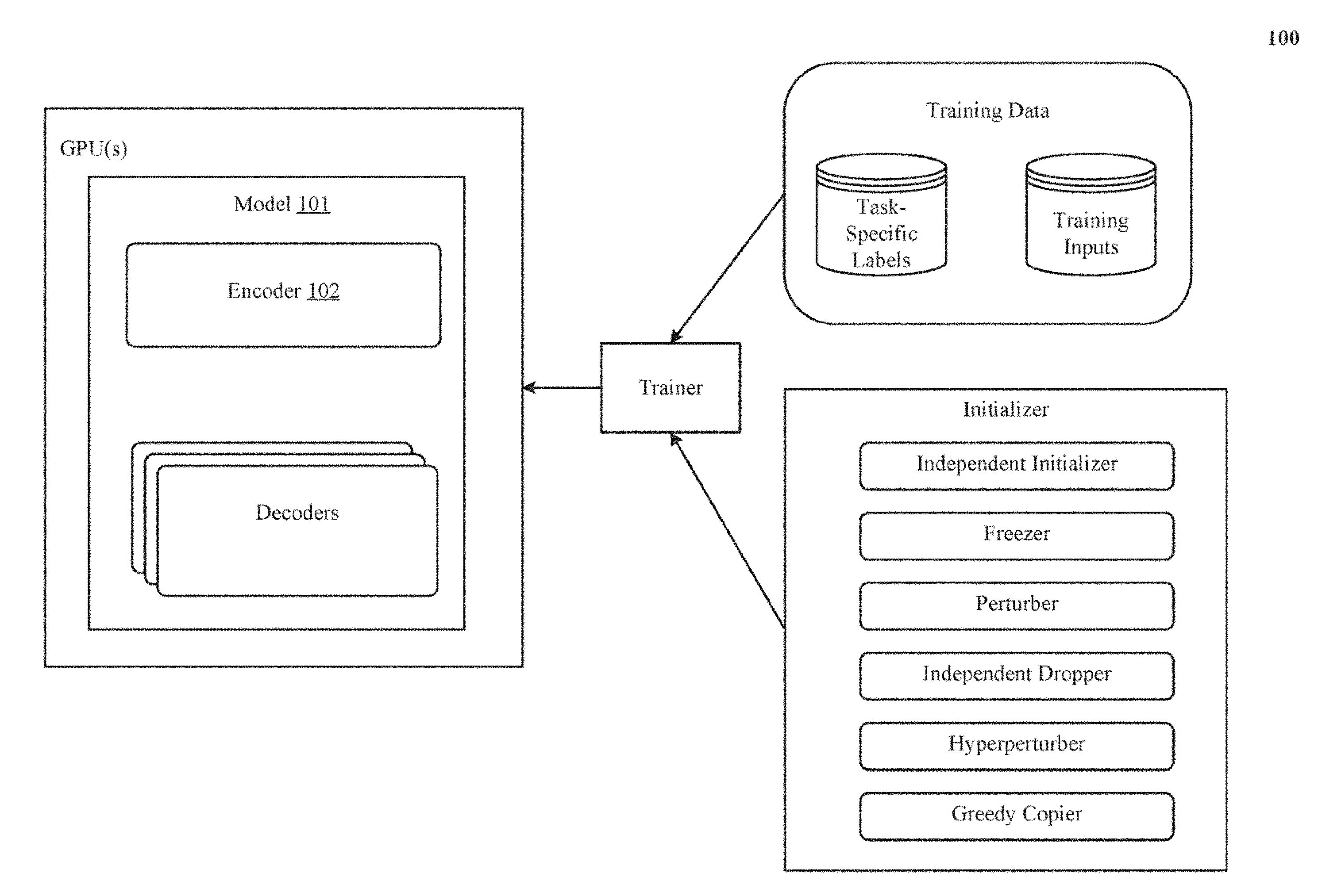
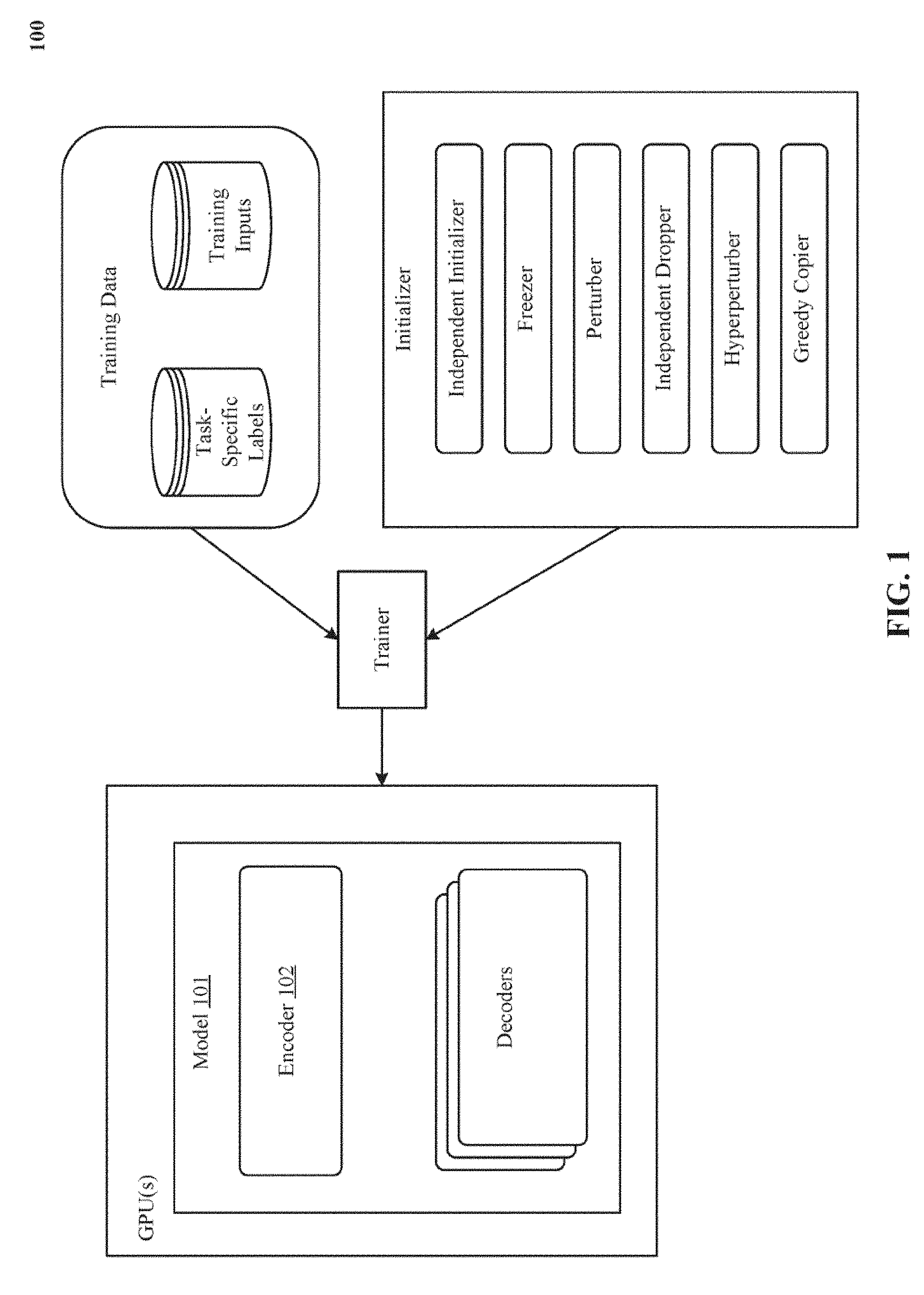
[0009] FIG. 1 is a block diagram that shows various aspects of the technology disclosed, including a model with an encoder and numerous decoders, training data, a trainer, and an initializer.
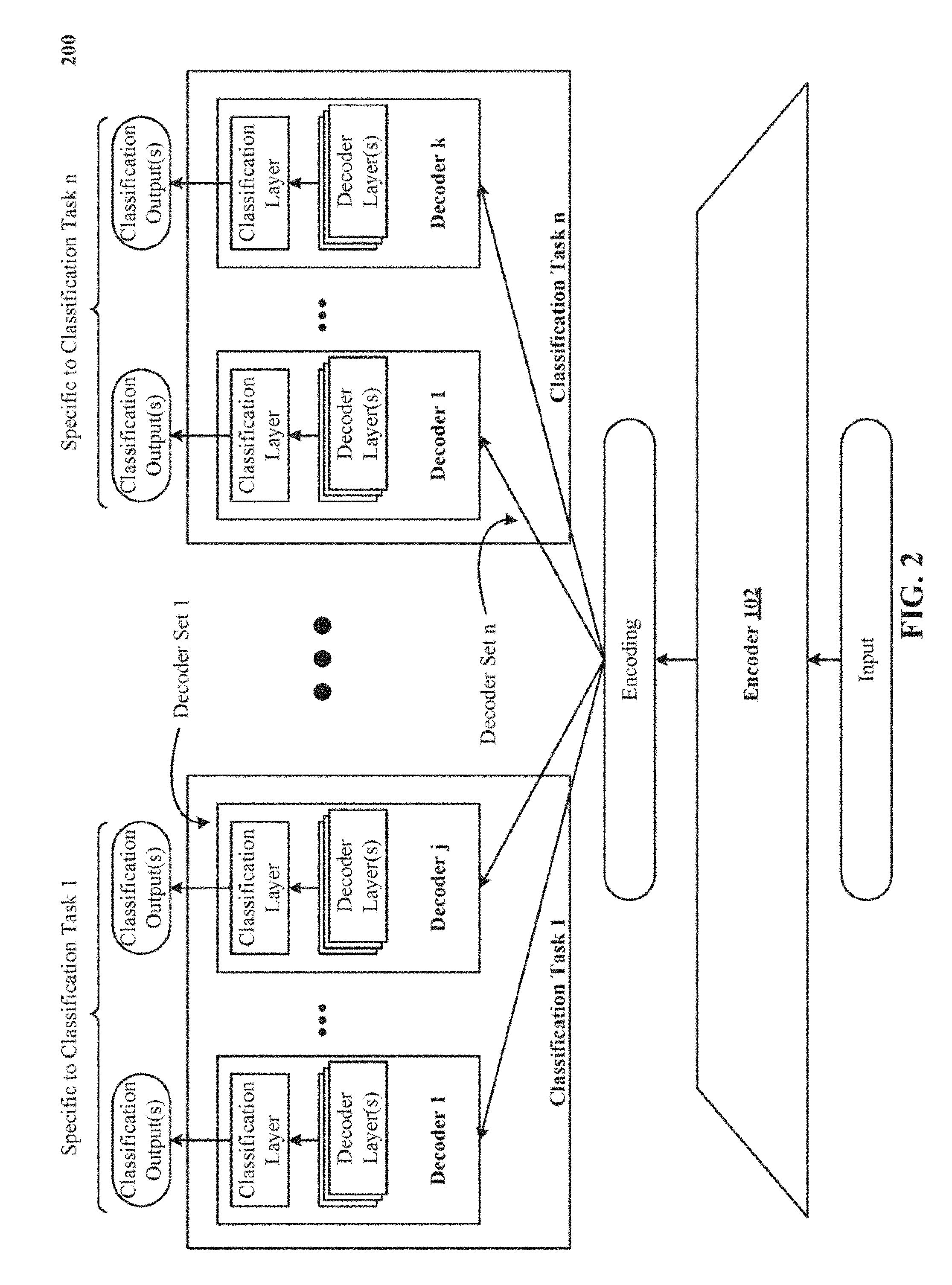
[0010] FIG. 2 illustrates one implementation of jointly training encoder-decoder pairs on corresponding classification tasks.
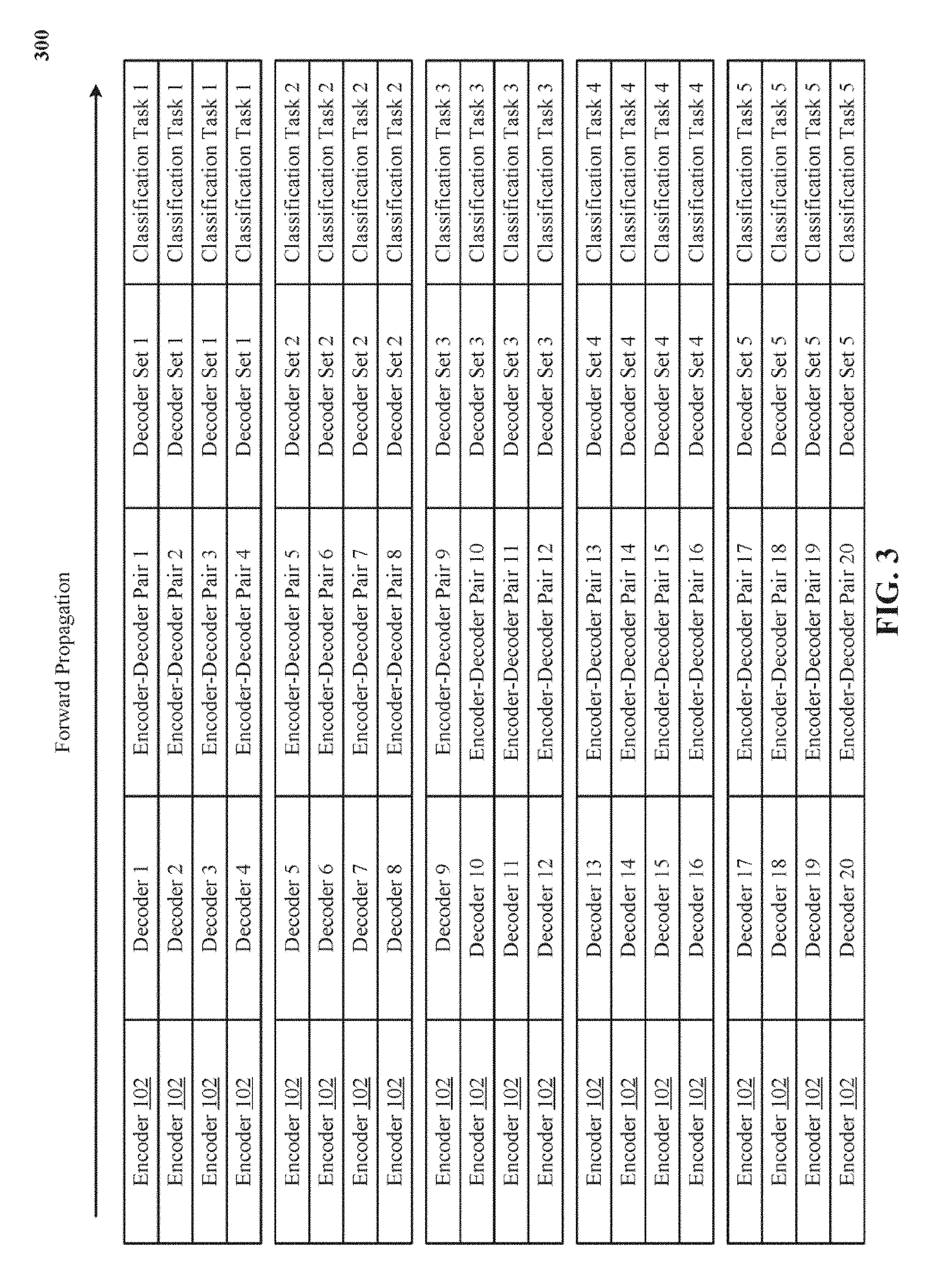
[0011] FIG. 3 depicts one forward propagation implementation of the encoder-decoder pairs operating independently of each other when performing the corresponding classification tasks.
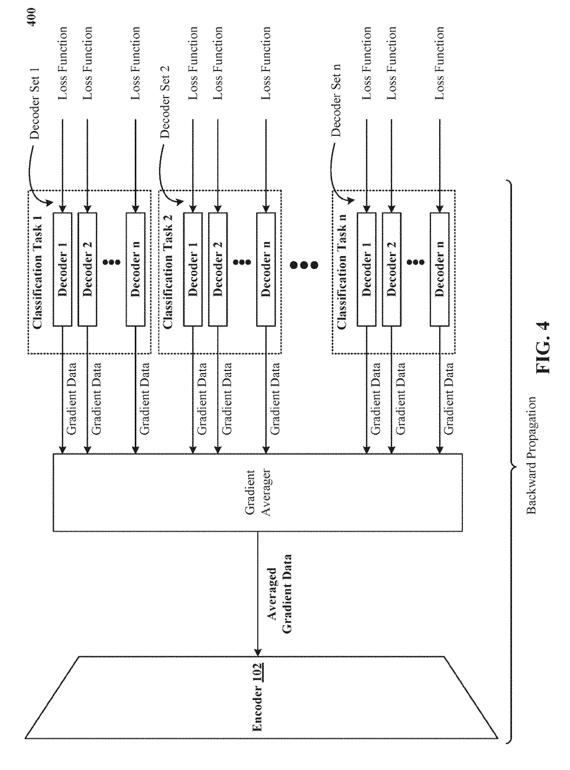
[0012] FIG. 4 illustrates one backward propagation implementation of modifying weights of the encoder by backpropagating through the encoder in dependence upon averaged gradient data determined for the decoders.
[0013] FIG. 5 is a simplified block diagram of a computer system that can be used to implement the technology disclosed.
[0014] FIG. 6 is an exemplary underlying model set-up for pseudo-task augmentation with two tasks.
[0015] FIG. 7 is an algorithm giving a high-level framework for applying explicit control to pseudo-task trajectories.
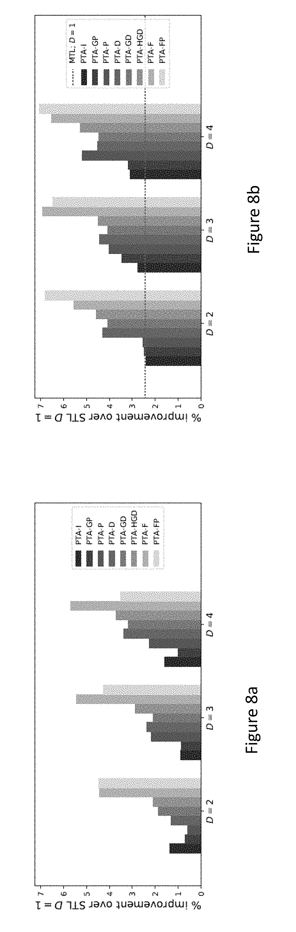
[0016] FIGS. 8a and 8b illustrate omniglot single-task (FIG. 8a) and multitask (FIG. 8b) learning results.
[0017] FIGS. 9a, 9b and 9c illustrate projections of pseudo-task trajectories, for runs of PTA-I, PTA-F, and PTA-HGD on IMDB.
[0018] FIG. 10 shows mean dropout schedule across all 400 pseudo-tasks in a run of PTA-HGD in accordance with an embodiment herein.
DESCRIPTION
[0019] The following discussion is presented to enable any person skilled in the art to make and use the technology disclosed, and is provided in the context of a particular application and its requirements. Various modifications to the disclosed implementations will be readily apparent to those skilled in the art, and the general principles defined herein may be applied to other implementations and applications without departing from the spirit and scope of the technology disclosed. Thus, the technology disclosed is not intended to be limited to the implementations shown, but is to be accorded the widest scope consistent with the principles and features disclosed herein.
[0020] The detailed description of various implementations will be better understood when read in conjunction with the appended drawings. To the extent that the figures illustrate diagrams of the functional blocks of the various implementations, the functional blocks are not necessarily indicative of the division between hardware circuitry. Thus, for example, one or more of the functional blocks (e.g., modules, processors, or memories) may be implemented in a single piece of hardware (e.g., a general purpose signal processor or a block of random access memory, hard disk, or the like) or multiple pieces of hardware. Similarly, the programs may be stand-alone programs, may be incorporated as subroutines in an operating system, may be functions in an installed software package, and the like. It should be understood that the various implementations are not limited to the arrangements and instrumentality shown in the drawings.
[0021] The processing engines and databases of the figures, designated as modules, can be implemented in hardware or software, and need not be divided up in precisely the same blocks as shown in the figures. Some of the modules can also be implemented on different processors, computers, or servers, or spread among a number of different processors, computers, or servers. In addition, it will be appreciated that some of the modules can be combined, operated in parallel or in a different sequence than that shown in the figures without affecting the functions achieved. The modules in the figures can also be thought of as flowchart steps in a method. A module also need not necessarily have all its code disposed contiguously in memory; some parts of the code can be separated from other parts of the code with code from other modules or other functions disposed in between.
System
[0022] FIG. 1 is a block diagram 100 that shows various aspects of the technology disclosed, including a model 101 with an encoder 102 and numerous decoders, training data, a trainer, and an initializer.
[0023] Encoder 102 is a processor that receives information characterizing input data and generates an alternative representation and/or characterization of the input data, such as an encoding. In particular, encoder 102 is a neural network such as a convolutional neural network (CNN), a multilayer perceptron, a feed-forward neural network, a recursive neural network, a recurrent neural network (RNN), a deep neural network, a shallow neural network, a fully-connected neural network, a sparsely-connected neural network, a convolutional neural network that comprises a fully-connected neural network (FCNN), a fully convolutional network without a fully-connected neural network, a deep stacking neural network, a deep belief network, a residual network, echo state network, liquid state machine, highway network, maxout network, long short-term memory (LSTM) network, recursive neural network grammar (RNNG), gated recurrent unit (GRU), pre-trained and frozen neural networks, and so on.
[0024] In implementations, encoder 102 includes individual components of a convolutional neural network (CNN), such as a one-dimensional (1D) convolution layer, a two-dimensional (2D) convolution layer, a three-dimensional (3D) convolution layer, a feature extraction layer, a dimensionality reduction layer, a pooling encoder layer, a subsampling layer, a batch normalization layer, a concatenation layer, a classification layer, a regularization layer, and so on.
[0025] In implementations, encoder 102 comprises learnable components, parameters, and hyperparameters that can be trained by backpropagating errors using an optimization algorithm. The optimization algorithm can be based on stochastic gradient descent (or other variations of gradient descent like batch gradient descent and mini-batch gradient descent). Some examples of optimization algorithms that can be used to train the encoder 102 are Momentum, Nesterov accelerated gradient, Adagrad, Adadelta, RMSprop, and Adam.
[0026] In implementations, encoder 102 includes an activation component that applies a non-linearity function. Some examples of non-linearity functions that can be used by the encoder 102 include a sigmoid function, rectified linear units (ReLUs), hyperbolic tangent function, absolute of hyperbolic tangent function, leaky ReLUs (LReLUs), and parametrized ReLUs (PReLUs).
[0027] In some implementations, encoder 102 can include a classification component, though it is not necessary. In preferred implementations, encoder 102 is a convolutional neural network (CNN) without a classification layer such as softmax or sigmoid. Some examples of classifiers that can be used by the encoder 102 include a multi-class support vector machine (SVM), a sigmoid classifier, a softmax classifier, and a multinomial logistic regressor. Other examples of classifiers that can be used by the encoder 102 include a rule-based classifier.
[0028] Some examples of the encoder 102 are: [0029] AlexNet [0030] ResNet [0031] Inception (various versions) [0032] WaveNet [0033] PixelCNN [0034] GoogLeNet [0035] ENet [0036] U-Net [0037] BN-NIN [0038] VGG [0039] LeNet [0040] DeepSEA [0041] DeepChem [0042] DeepBind [0043] DeepMotif [0044] FIDDLE [0045] DeepLNC [0046] DeepCpG [0047] DeepCyTOF [0048] SPINDLE
[0049] In model 101, the encoder 102 produces an output, referred to herein as "encoding", which is fed as input to each of the decoders. When the encoder 102 is a convolutional neural network (CNN), the encoding is convolution data. When the encoder 102 is a recurrent neural network (RNN), the encoding is hidden state data.
[0050] Each decoder is a processor that receives, from the encoder 102, information characterizing input data (such as the encoding) and generates an alternative representation and/or characterization of the input data, such as classification scores. In particular, each decoder is a neural network such as a convolutional neural network (CNN), a multilayer perceptron, a feed-forward neural network, a recursive neural network, a recurrent neural network (RNN), a deep neural network, a shallow neural network, a fully-connected neural network, a sparsely-connected neural network, a convolutional neural network that comprises a fully-connected neural network (FCNN), a fully convolutional network without a fully-connected neural network, a deep stacking neural network, a deep belief network, a residual network, echo state network, liquid state machine, highway network, maxout network, long short-term memory (LSTM) network, recursive neural network grammar (RNNG), gated recurrent unit (GRU), pre-trained and frozen neural networks, and so on.
[0051] In implementations, each decoder includes individual components of a convolutional neural network (CNN), such as a one-dimensional (1D) convolution layer, a two-dimensional (2D) convolution layer, a three-dimensional (3D) convolution layer, a feature extraction layer, a dimensionality reduction layer, a pooling encoder layer, a subsampling layer, a batch normalization layer, a concatenation layer, a classification layer, a regularization layer, and so on.
[0052] In implementations, each decoder comprises learnable components, parameters, and hyperparameters that can be trained by backpropagating errors using an optimization algorithm. The optimization algorithm can be based on stochastic gradient descent (or other variations of gradient descent like batch gradient descent and mini-batch gradient descent). Some examples of optimization algorithms that can be used to train each decoder are Momentum, Nesterov accelerated gradient, Adagrad, Adadelta, RMSprop, and Adam.
[0053] In implementations, each decoder includes an activation component that applies a non-linearity function. Some examples of non-linearity functions that can be used by each decoder include a sigmoid function, rectified linear units (ReLUs), hyperbolic tangent function, absolute of hyperbolic tangent function, leaky ReLUs (LReLUs), and parametrized ReLUs (PReLUs).
[0054] In implementations, each decoder includes a classification component. Some examples of classifiers that can be used by each decoder include a multi-class support vector machine (SVM), a sigmoid classifier, a softmax classifier, and a multinomial logistic regressor. Other examples of classifiers that can be used by each decoder include a rule-based classifier.
[0055] The numerous decoders can all be the same type of neural networks with matching architectures, such as fully-connected neural networks (FCNN) with an ultimate sigmoid or softmax classification layer. In other implementations, they can differ based on the type of the neural networks. In yet other implementations, they can all be the same type of neural networks with different architectures.
Joint Training
[0056] FIG. 2 illustrates one implementation of jointly training 200 encoder-decoder pairs on corresponding classification tasks. FIG. 2 also shows how model 101 includes multiple processing pipeline in which an input (such as an image) is first processed through the encoder 102 to generate the encoding, and the encoding is then separately fed as input to each of the different decoders. This way, numerous encoder-decoder pairs are formed; all of which have the same underlying encoder 102.
[0057] Note that the processing through the same underlying encoder 102 to produce the encoding occurs only once during a given forward pass step; however, multiple processing steps occur independently and concurrently in each of the different decoders during the given forward pass step to produce respective classification outputs, as discussed below.
[0058] Similarly, multiple processing steps occur independently and concurrently in each of the different decoders during a given backward pass step, as discussed below.
[0059] As used herein, "concurrently" or "in parallel" does not require exact simultaneity. It is sufficient if the processing of one of the decoders begins before the processing of another of the decoder completes.
[0060] FIG. 2 further shows that the numerous decoders are grouped into sets of decoders (or decoder sets) in dependence upon corresponding classification tasks. Consider that the model 101 has a total of 400 decoders and there are 40 classification tasks to be performed, then groups of 10 decoders can be grouped in 40 decoder sets such decoders in the same decoder set perform the same classification task; of course in conjunction with the same underlying encoder 102. In other implementations, the number of grouped decoders can vary from decoder set to decoder set.
[0061] Regarding the classification tasks, they can be distinct and/or related. For example, each classification task can be to predict a different facial attribute in the same image such as age, bags under eye, full lips, smiling, prominent nose, blonde hair, bald, wavy hair, goatee, mustache, full face, large chin, lipstick, and eyeglasses. In such a case, a single image, annotated with numerous ground truths corresponding to the respective classification task, can be fed as input to the encoder 102 and the performance of the model 101 can be determined accordingly by computing an error using a loss function. In another implementation, each classification task can be to predict a different alphabet letter from among the twenty-seven alphabet letters or to predict a different numerical digit from among the ten numeric digits. In such cases, twenty-seven images or ten images, each annotated with a single ground truth corresponding to a respective alphabet letter or numerical digit, can be fed in parallel as input to the encoder 102 during a single forward pass iteration and the performance of the model 101 can determined accordingly by computing an error using a loss function. In yet other implementations, the classification tasks can be different natural language processing tasks such as part-of-speech (POS) tagging, chunking, dependency parsing, and sentiment analysis.
[0062] It is important to note that even though different decoder sets perform different classification tasks and decoders in the same decoder set perform the same classification task, each of the decoders operates independently of each other but in conjunction with the same underlying encoder 102. Turning to FIG. 2 again, consider that classification task 1 is to evaluate an input image and predict the age of the person in the image and classification task n is to evaluate the same image and predict whether the person in the image is wearing eyeglasses.
[0063] Now, as illustrated, decoders 1 and j in the decoder set 1 will separately receive the encoding from the encoder 102 and process it through their respective decoder layers and classification layers and generate separate classification outputs on the likely age of the person in the image. The classification outputs are specific to the classification task 1 being performed by the decoders 1 and j in the decoder set 1. In other words, they are specific to the classes defined for the classification task 1 being performed by the decoders 1 and j in the decoder set 1 (e.g., a young class and an old class or a softmax distribution between 1 year and 100 years or a sigmoid value between 0 and 1 with 0 representing young and 1 representing old).
[0064] Thus, even though decoders 1 and j in the decoder set 1 performed the same classification task 1, they performed it independently of each other or of any other decoder in the model 101. As a result, the forward propagation and the backward propagation also occurs separately and independently in the decoders 1 and j (and all other decoders in general).
[0065] Decoders 1 and k in the decoder set n operate in parallel to, concurrently, or simultaneously to decoders 1 and j in the decoder set 1, but, independently and in conjunction with the same underlying encoder 102, to perform a different classification task n of predicting whether the person in the image is wearing eyeglasses.
[0066] Now, as illustrated, decoders 1 and k in the decoder set n will separately receive the encoding from the encoder 102 and process it through their respective decoder layers and classification layers and generate separate classification outputs on whether the person in the image is wearing eyeglasses. The classification outputs are specific to the classification task n being performed by the decoders 1 and k in the decoder set n. In other words, they are specific to the classes defined for the classification task n being performed by the decoders 1 and k in the decoder set n (e.g., an eyeglasses class and a no eyeglasses class).
Forward Propagation
[0067] FIG. 3 depicts one forward propagation implementation of the encoder-decoder pairs 1-20 operating 300 independently of each other when performing the corresponding classification tasks 1-5. In FIG. 3, as a way of example, twenty encoder-decoder pairs, each with the same underlying encoder 102 but a different decoder perform corresponding classification tasks 1, 2, 3, 4, or 5. Note that multiple decoders that are grouped in the same decoder set independently perform the same classification task. Also, decoders that are grouped in different decoder sets independently perform different classification tasks.
Backward Propagation
[0068] FIG. 4 illustrates one backward propagation implementation of modifying weights of the encoder by backpropagating 400 through the encoder 102 in dependence upon averaged gradient data determined for the decoders. For each of one thousand to millions of backpropagation iterations complemented by forward pass evaluation of training examples, gradient data for each of the decoders is determined in dependence upon a loss function. A gradient averager, shown in FIG. 4, averages the gradient data determined for the decoders.
[0069] The averaged gradient data is then backpropagated through the encoder 102 to determine gradient data for the encoder 102. Weights of the encoder 102 are then updated in dependence upon the gradient data determined for the encoder 102.
[0070] Receiving an average of gradients from decoders that are configured to perform different classification tasks trains the encoder 102 to generate an encoding that is suitable for a variety of classification tasks. In other words, encoder 102 becomes better at generating an encoding that generalizes for a wider range or pool of classification tasks. This makes encoder 102 more robust to feature diversity typically seen in real-world data.
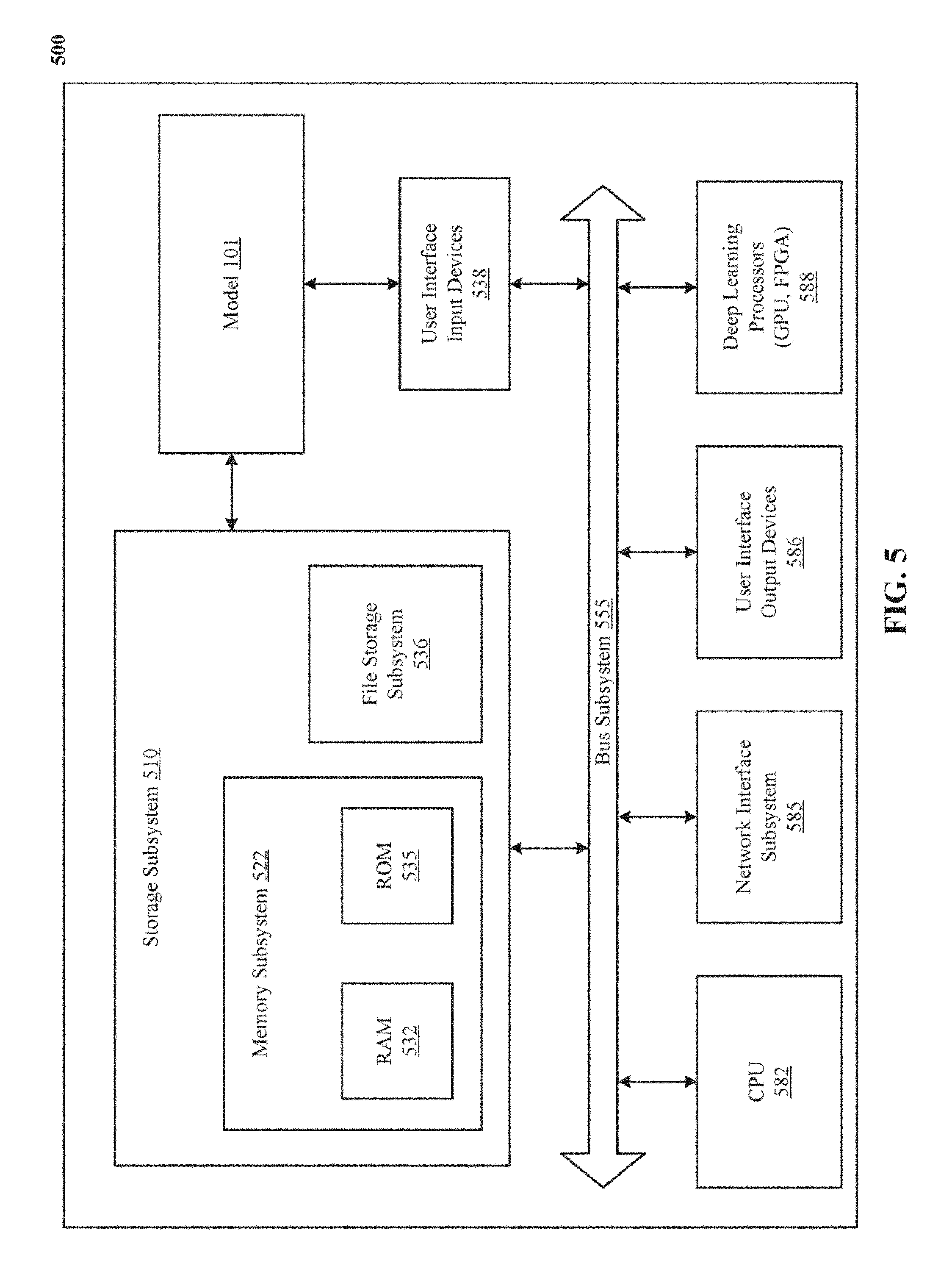
Computer System
[0071] FIG. 5 is a simplified block diagram of a computer system 500 that can be used to implement the technology disclosed. Computer system 500 includes at least one central processing unit (CPU) 572 that communicates with a number of peripheral devices via bus subsystem 555. These peripheral devices can include a storage subsystem 510 including, for example, memory devices and a file storage subsystem 536, user interface input devices 538, user interface output devices 576, and a network interface subsystem 574. The input and output devices allow user interaction with computer system 500. Network interface subsystem 574 provides an interface to outside networks, including an interface to corresponding interface devices in other computer systems.
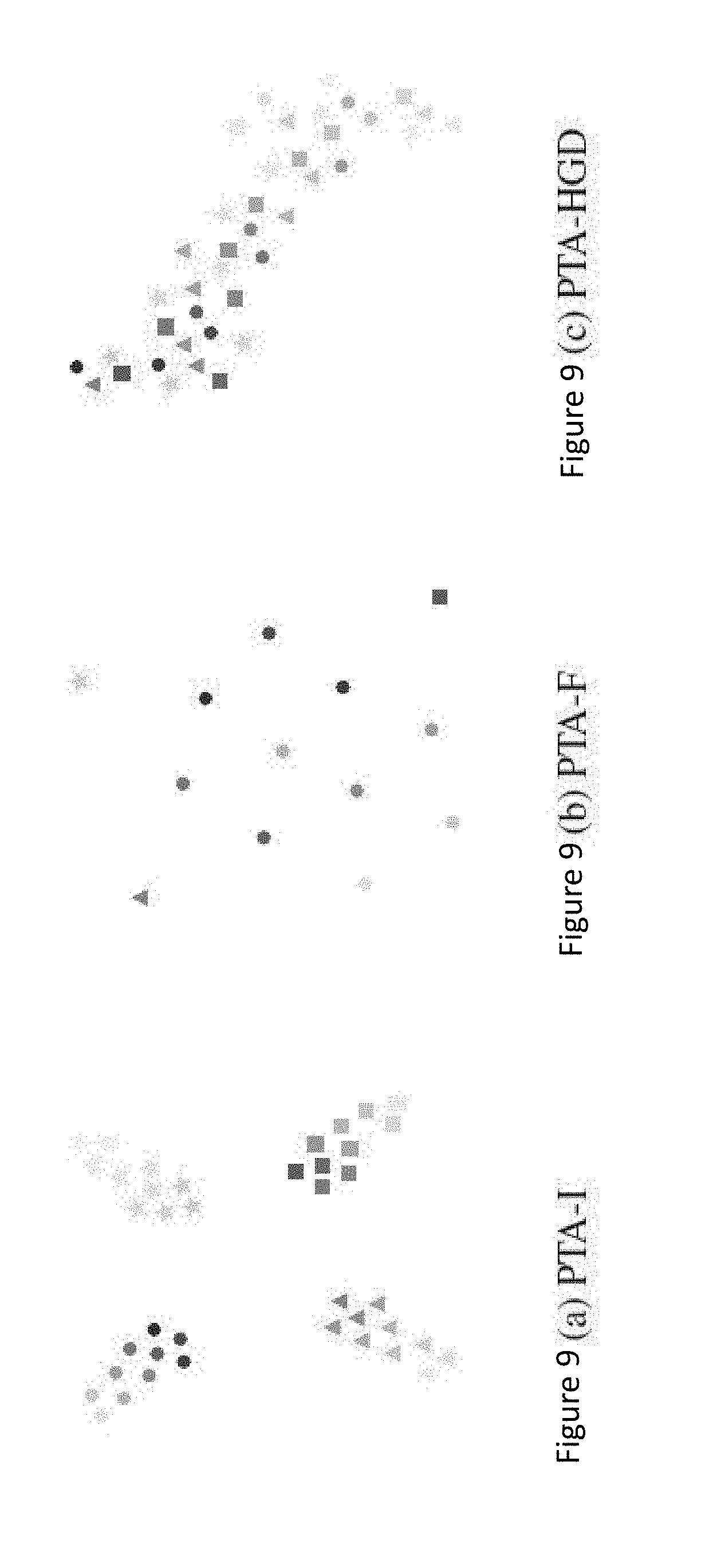
[0072] In one implementation, the model 101 is communicably linked to the storage subsystem 510 and the user interface input devices 538.
[0073] User interface input devices 538 can include a keyboard; pointing devices such as a mouse, trackball, touchpad, or graphics tablet; a scanner; a touch screen incorporated into the display; audio input devices such as voice recognition systems and microphones; and other types of input devices. In general, use of the term "input device" is intended to include all possible types of devices and ways to input information into computer system 500.
[0074] User interface output devices 576 can include a display subsystem, a printer, a fax machine, or non-visual displays such as audio output devices. The display subsystem can include an LED display, a cathode ray tube (CRT), a flat-panel device such as a liquid crystal display (LCD), a projection device, or some other mechanism for creating a visible image. The display subsystem can also provide a non-visual display such as audio output devices. In general, use of the term "output device" is intended to include all possible types of devices and ways to output information from computer system 500 to the user or to another machine or computer system.
[0075] Storage subsystem 510 stores programming and data constructs that provide the functionality of some or all of the modules and methods described herein. Subsystem 578 can be graphics processing units (GPUs) or field-programmable gate arrays (FPGAs).
[0076] Memory subsystem 522 used in the storage subsystem 510 can include a number of memories including a main random access memory (RAM) 532 for storage of instructions and data during program execution and a read only memory (ROM) 534 in which fixed instructions are stored. A file storage subsystem 536 can provide persistent storage for program and data files, and can include a hard disk drive, a floppy disk drive along with associated removable media, a CD-ROM drive, an optical drive, or removable media cartridges. The modules implementing the functionality of certain implementations can be stored by file storage subsystem 536 in the storage subsystem 510, or in other machines accessible by the processor.
[0077] Bus subsystem 555 provides a mechanism for letting the various components and subsystems of computer system 500 communicate with each other as intended. Although bus subsystem 555 is shown schematically as a single bus, alternative implementations of the bus subsystem can use multiple busses.
[0078] Computer system 500 itself can be of varying types including a personal computer, a portable computer, a workstation, a computer terminal, a network computer, a television, a mainframe, a server farm, a widely-distributed set of loosely networked computers, or any other data processing system or user device. Due to the ever-changing nature of computers and networks, the description of computer system 500 depicted in FIG. 5 is intended only as a specific example for purposes of illustrating the preferred embodiments of the present invention. Many other configurations of computer system 500 are possible having more or less components than the computer system depicted in FIG. 5.
Particular Implementations
[0079] In one implementation, we describe a system and various implementations of multi-task (MTL) learning using an encoder-decoders architecture. One or more features of an implementation can be combined with the base implementation. Implementations that are not mutually exclusive are taught to be combinable. One or more features of an implementation can be combined with other implementations. This disclosure periodically reminds the user of these options. Omission from some implementations of recitations that repeat these options should not be taken as limiting the combinations taught in the preceding sections--these recitations are hereby incorporated forward by reference into each of the following implementations.
[0080] In one implementation, the technology disclosed presents a neural network-based model. The model is coupled to memory and runs on one or more parallel processors.
[0081] The model has an encoder that processes an input and generates an encoding.
[0082] The model has numerous decoders. The decoders are grouped into sets of decoders in dependence upon corresponding classification tasks. The decoders respectively receive the encoding as input from the encoder, thereby forming encoder-decoder pairs which operate independently of each other when performing the corresponding classification tasks. The decoders respectively process the encoding and produce classification scores for classes defined for the corresponding classification tasks.
[0083] A trainer jointly trains the encoder-decoder pairs over one thousand to millions of backpropagation iterations to perform the corresponding classification tasks.
[0084] This system implementation and other systems disclosed optionally include one or more of the following features. System can also include features described in connection with methods disclosed. In the interest of conciseness, alternative combinations of system features are not individually enumerated. Features applicable to systems, methods, and articles of manufacture are not repeated for each statutory class set of base features. The reader will understand how features identified in this section can readily be combined with base features in other statutory classes.
[0085] The trainer is further configured to comprise a forward pass stage that processes training inputs through the encoder and resulting encodings through the decoders to compute respective activations for each of the training inputs, a backward pass stage, that, over each of the one thousand to millions of backpropagation iterations, determines gradient data for the decoders for each of the training inputs in dependence upon a loss function, averages the gradient data determined for the decoders, and determines gradient data for the encoder by backpropagating the averaged gradient data through the encoder, an update stage that modifies weights of the encoder in dependence upon the gradient data determined for the encoder, and a persistence stage that, upon convergence after a final backpropagation iteration, persists in the memory the modified weights of the encoder derived by the training to be applied to future classification tasks.
[0086] The model is further configured to use a combination of the modified weights of the encoder derived by the training and modified weights of a particular one of the decoders derived by the training to perform a particular one of the classification tasks on inference inputs. The inference inputs are processed by the encoder to produce encodings, followed by the particular one of the decoders processing the encodings to output classification scores for classes defined for the particular one of the classification tasks.
[0087] The model is further configured to use a combination of the modified weights of the encoder derived by the training and modified weights of two or more of the decoders derived by the training to respectively perform two or more of the classification tasks on inference inputs. The inference inputs are processed by the encoder to produce encodings, followed by the two or more of the decoders respectively processing the encodings to output classification scores for classes defined for the two or more of the classification tasks.
[0088] Each training input is annotated with a plurality of task-specific labels for the corresponding classification tasks. A plurality of training inputs for the corresponding classification tasks are fed in parallel to the encoder as input in each forward pass iteration. Each training input is annotated with a task-specific label for a corresponding classification task.
[0089] The loss function is cross entropy that uses either a maximum likelihood objective function, a policy gradient function, or both.
[0090] The encoder is a convolutional neural network (abbreviated CNN) with a plurality of convolution layers arranged in a sequence from lowest to highest. The encoding is convolution data.
[0091] Each decoder further comprises at least one decoder layer and at least one classification layer. The decoder is a fully-connected neural network (abbreviated FCNN) and the decoder layer is a fully-connected layer. The classification layer is a sigmoid classifier. The classification layer is a softmax classifier.
[0092] The encoder is a recurrent neural network (abbreviated RNN), including long short-term memory (LSTM) network or gated recurrent unit (GRU) network. The encoding is hidden state data. The encoder is a fully-connected neural network (abbreviated FCNN) with at least one fully-connected layer.
[0093] Each decoder is a recurrent neural network (abbreviated RNN), including long short-term memory (LSTM) network or gated recurrent unit (GRU) network. Each decoder is a convolutional neural network (abbreviated CNN) with a plurality of convolution layers arranged in a sequence from lowest to highest.
[0094] At least some of the decoders are of a first neural network type, at least some of the decoders are of a second neural network type, and at least some of the decoders are of a third neural network type. At least some of the decoders are convolutional neural networks (abbreviated CNNs) with a plurality of convolution layers arranged in a sequence from lowest to highest, at least some of the decoders are recurrent neural networks (abbreviated RNNs), including long short-term memory (LSTM) networks or gated recurrent unit (GRU) networks, and at least some of the decoders are fully-connected neural networks (abbreviated FCNNs).
[0095] The input, the training inputs, and the inference inputs are image data. The input, the training inputs, and the inference inputs are text data. The input, the training inputs, and the inference inputs are genomic data.
[0096] The model is further configured to comprise an independent initializer that initializes the decoders with random weights.
[0097] The model is further configured to comprise a freezer that freezes weights of some decoders for certain number of backpropagation iterations while updating weights of at least one high performing decoder among the decoders over the certain number of backpropagation iterations. The high performing decoder is identified based on performance on validation data.
[0098] The model is further configured to comprise a perturber that periodically perturbs weights of the decoders after certain number of backpropagation iterations by adding random noise to the weights.
[0099] The model is further configured to comprise an independent dropper that periodically and randomly drops out weights of the decoders after certain number of backpropagation iterations.
[0100] The model is further configured to comprise a hyperperturber that periodically perturbs hyperparameters of the decoders after certain number of backpropagation iterations by randomly changing a rate at which weights of the decoders are randomly dropped out.
[0101] The model is further configured to comprise a greedy coper that identifies at least one high performing decoder among the decoders after every certain number of backpropagation iterations and copies weights and hyperparameters of the high performing decoder to the other decoders. The high performing decoder is identified based on performance on validation data.
[0102] Other implementations may include a non-transitory computer readable storage medium storing instructions executable by a processor to perform actions of the system described above. Each of the features discussed in the particular implementation section for other implementations apply equally to this implementation. As indicated above, all the other features are not repeated here and should be considered repeated by reference.
[0103] In one implementation, the technology disclosed presents a neural network-implemented method.
[0104] The method includes processing an input through an encoder and generating an encoding.
[0105] The method includes processing the encoding through numerous decoders and producing classification scores for classes defined for corresponding classification tasks. The decoders are grouped into sets of decoders in dependence upon the corresponding classification tasks and respectively receive the encoding as input from the encoder, thereby forming encoder-decoder pairs which operate independently of each other.
[0106] The method includes jointly training the encoder-decoder pairs over one thousand to millions of backpropagation iterations to perform the corresponding classification tasks.
[0107] Other implementations may include a non-transitory computer readable storage medium (CRM) storing instructions executable by a processor to perform the method described above. Yet another implementation may include a system including memory and one or more processors operable to execute instructions, stored in the memory, to perform the method described above. Each of the features discussed in the particular implementation section for other implementations apply equally to this implementation. As indicated above, all the other features are not repeated here and should be considered repeated by reference.
[0108] In another implementation, the multi-task (MTL) process is adapted to the single-task learning (STL) case, i.e., when only a single task is available for training. The method is formalized as pseudo-task augmentation (PTA), in which a single task has multiple distinct decoders projecting the output of the shared structure to task predictions. By training the shared structure to solve the same problem in multiple ways, PTA simulates the effect of training towards distinct but closely-related tasks drawn from the same universe. Theoretical justification shows how training dynamics with multiple pseudo-tasks strictly subsumes training with just one, and a class of algorithms is introduced for controlling pseudo-tasks in practice.
[0109] In an array of experiments discussed further herein, PTA is shown to significantly improve performance in single-task settings. Although different variants of PTA traverse the space of pseudo-tasks in qualitatively different ways, they all demonstrate substantial gains. As discussed below, experiments also show that when PTA is combined with MTL, further improvements are achieved, including state-of-the-art performance on the CelebA dataset. In other words, although PTA can be seen as a base case of MTL, PTA and MTL have complementary value in learning more generalizable models. The conclusion is that pseudo-task augmentation is an efficient, reliable, and broadly applicable method for boosting performance in deep learning systems.
[0110] The following method combines the benefits of the joint training of models for multiple tasks and separate training of multiple models for single tasks to train multiple models that share underlying parameters and sample complementary high-performing areas of the model space to improve single task performance. In this description, first, the classical deep MTL approach is extended to the case of multiple decoders per task. Then, the concept of a pseudo-task is introduced, and increased training dynamics under multiple pseudo-tasks is demonstrated. Finally, practical methods for controlling pseudo-tasks during training are described and compared empirically.
[0111] The most common approach to deep MTL is still the "classical" approach, in which all layers are shared across all tasks up to a high level, after which each task learns a distinct decoder that maps high-level points to its task-specific output space. Even when more sophisticated methods are developed, the classical approach is often used as a baseline for comparison. The classical approach is also computationally efficient, in that the only additional parameters beyond a single task model are in the additional decoders. Thus, when applying ideas from deep MTL to single-task multi-model learning, the classical approach is a natural starting point. Consider the case where there are T distinct true tasks, but now let there be D decoders for each task. Then, the model for the dth decoder of the tth task is given by (Eq. 1):
y.sub.tdi=.sub.td((x.sub.ti; .theta.); .theta..sub.td),
In which a joint model is decomposed into an underlying model F (parameterized by .theta.F) that is shared across all tasks, and task-specific decoders D.sub.t (parameterized by .theta..sub.Dt) for each task. And the overall loss for the joint model is given by (Eq. 2):
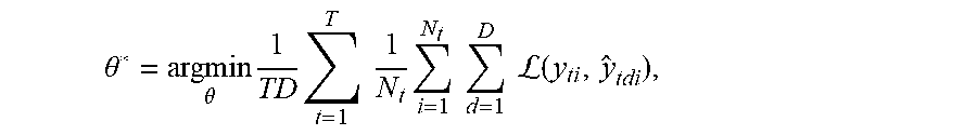
.theta. * = argmin .theta. 1 TD t = 1 T 1 N t i = 1 N t d = 1 D L ( y ti , y ^ tdi ) , ##EQU00001##
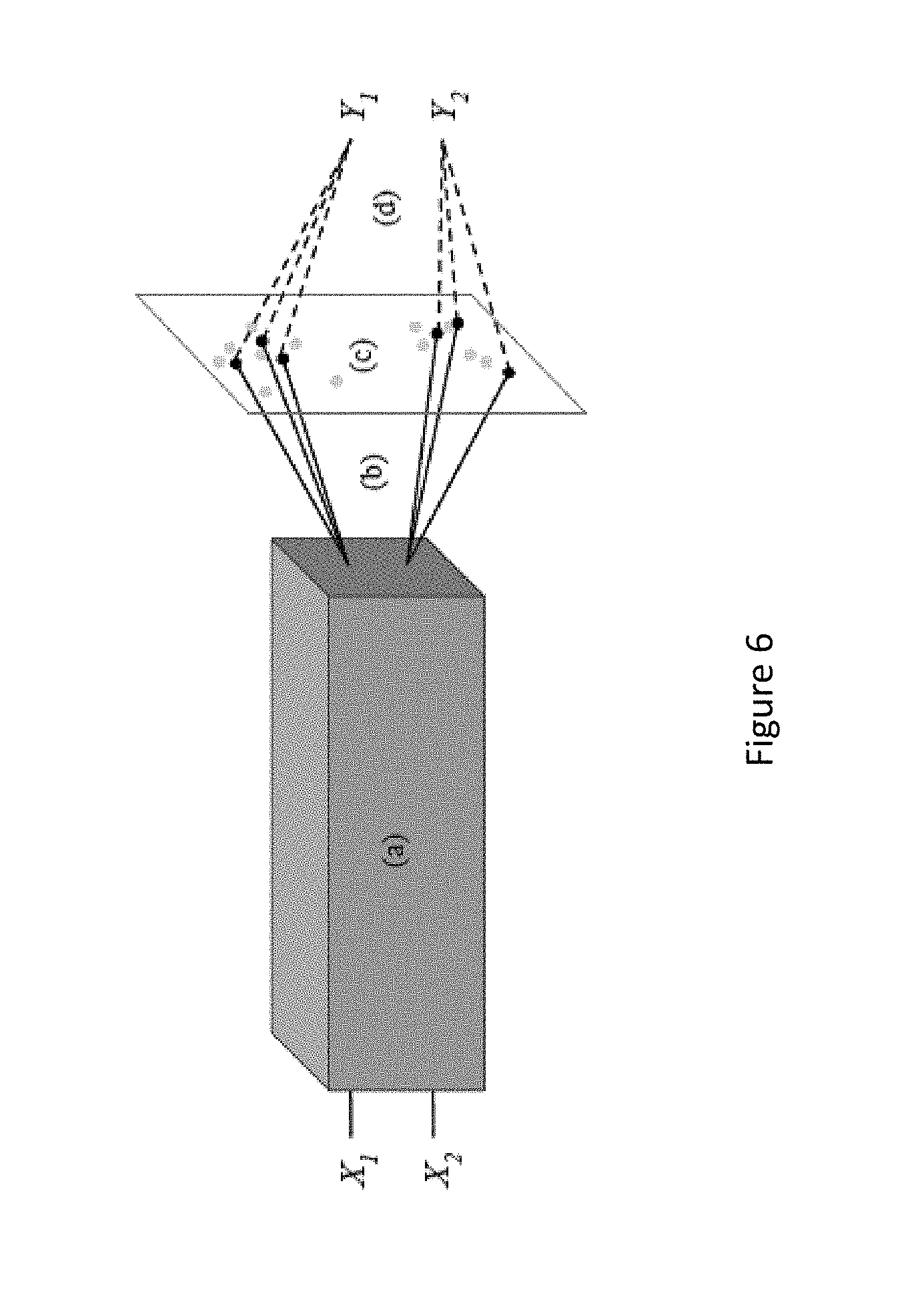
where .theta.=({{.theta..sub.td}.sub.d=1.sup.D}.sub.t=1.sup.T, .theta.). In the same way as the classical approach to MTL encourages F to be more general and robust by requiring it to support multiple tasks, here F is required to support solving the same task in multiple ways. A visualization of a resulting joint model is shown in FIG. 6 which illustrates a general setup for pseudo-task augmentation with two tasks. In FIG. 6 (a) is the underlying model wherein all task inputs are embedded through an underlying model that is completely shared; (b) shows multiple decoders, wherein each task has multiple decoders (solid black lines) each projecting the embedding to a distinct classification layer; (c) shows parallel traversal of model space, wherein the underlying model coupled with a decoder defines a task model and task models populate a model space, with current models shown as black dots and previous models shown as gray dots; and (d) shows multiple loss signals. Each current task model receives a distinct loss to compute its distinct gradient. A task coupled with a decoder and its parameters defines a pseudo-task for the underlying model. A theme in MTL is that models for related tasks will have similar decoders, as implemented by explicit regularization. Similarly, in Eq. 2, through training, two decoders for the same task will instantiate similar models, and, as long as they do not converge completely to equality, they will simulate the effect of training with multiple closely-related tasks.
[0112] Notice that the innermost summation in Eq. 2 is over decoders. This calculation is computationally efficient: because each decoder for a given task takes the same input, F(x.sub.ti) (usually the most expensive part of the model) need only be computed once per sample (and only once over all tasks if all tasks share x.sub.ti). However, when evaluating the performance of a model, since each decoder induces a distinct model for a task, what matters is not the average over decoders, but the best performing decoder for each task, i.e., (Eq. 3)
.theta. eval * = argmin .theta. 1 T t = 1 T 1 N t argmin d .di-elect cons. 1 D i = 1 N t L ( y ti , y ^ tdi ) . ##EQU00002##
Eq. 2 is used in training because it is smoother; Eq. 3 is used for model validation, and to select the best performing decoder for each task from the final joint model. This decoder is then applied to future data, e.g., a holdout set. Once the models are trained, in principle they form a set of distinct and equally powerful models for each task. It may therefore be tempting to ensemble them for evaluation, i.e., (Eq. 4):
.theta. ens * = argmin .theta. 1 T t = 1 T 1 N t i = 1 N t L ( y ti , 1 D d = 1 D y ^ tdi ) . ##EQU00003##
However, with linear decoders, training with Eq. 4 is equivalent to training with a single decoder for each task, while training with Eq. 2 with multiple decoders yields more expressive training dynamics.
[0113] Following the intuition that training F with multiple decoders amounts to solving the task in multiple ways, each "way" is defined by a pseudo-task (Eq. 5):
(.sub.td, .theta..sub.td, {x.sub.ti, y.sub.ti}.sub.i=1.sup.N.sup.t)
Of the true underlying task {x.sub.ti, y.sub.ti}.sub.i=1.sup.N.sup.t. It is termed a pseudo-task because it derives from a true task, but has no fixed labels. That is, for any fixed .theta..sub.td, there are potentially many optimal outputs for F(x.sub.ij). When D>1, training F amounts to training each task with multiple pseudo-tasks for each task at each gradient update step. This process is the essence of PTA.
[0114] As a first step, we consider linear decoders, i.e. each .theta..sub.td consists of a single dense layer of weights (any following nonlinearity can be considered part of the loss function). Similarly, with linear decoders, distinct pseudo-tasks for the same task simulate multiple closely-related tasks. When .theta..sub.td are considered fixed, the learning problem (Eq. 2) reduces to (Eq. 6):
.theta. * = argmin .theta. 1 TD t = 1 T 1 N t i = 1 N t d = 1 D L ( y ti , y ^ tdi ) . ##EQU00004##
In other words, although the overall goal is to learn models for T tasks, F is at each step optimized towards DT pseudotasks. Thus, training with multiple decoders may yield positive effects similar to training with multiple true tasks.
[0115] After training, the best model for a given task is selected from the final joint model, and used as the final model for that task (Eq. 3). Of course, using multiple decoders with identical architectures for a single task does not make the final learned predictive models more expressive. It is therefore natural to ask whether including additional decoders has any fundamental effect on learning dynamics. It turns out that even in the case of linear decoders, the training dynamics of using multiple pseudo-tasks strictly subsumes using just one.
[0116] Accordingly, given that a set of pseudotasks S1 simulates another S2 on F if for all .theta.F the gradient update to .theta.F when trained with S1 is equal to that with S2, there exist differentiable functions F and sets of pseudo-tasks of a single task that cannot be simulated by a single pseudo-task of that task, even when all decoders are linear.
[0117] Consider a task with a single sample (x; y), where y is a scalar. Suppose L (from Eq. 6) computes mean squared error, F has output dimension M, and all decoders are linear, with bias terms omitted for clarity. D.sub.d is then completely specified by the vector w.sub.d=w.sub.d.sup.1, w.sub.d.sup.2, . . . , w.sub.d.sup.M.sup.T. Suppose parameter updates are performed by gradient descent. The update rule for .theta..sub.F with fixed decoders {.sub.d}.sub.d=1.sup.D and learning rate .alpha. is then given by Eq. 7:
.theta. := .theta. - .alpha. d = 1 D .gradient. ( y - w d ( x ; .theta. ) ) 2 . ##EQU00005##
For a single fixed decoder to yield equivalent behavior, it must have equivalent update steps. The goal then is to choose (x; y), , {.theta..sub.k}.sub.k=1.sup.K, {w.sub.d}.sub.d=1.sup.D, and .alpha.>0, such that there are no w.sub.o, .gamma.>0, for which .A-inverted.k(Eq. 8)
.alpha. d = 1 D .gradient. ( y - w d ( x ; .theta. k ) ) 2 = .gamma. .gradient. ( y - w o ( x ; .theta. k ) ) 2 .alpha. d = 1 D 2 ( y - w d ( x ; .theta. k ) ) w d J ( x ; .theta. k ) = 2 .gamma. ( y - w o ( x ; .theta. k ) ) w o J ( x ; .theta. k ) , ##EQU00006##
where J.sub.F is the Jacobian of F. By choosing F and {.theta..sub.k}.sub.k=1.sup.K so that all J.sub.F(x; .theta..sub.k) have full row rank, Eq. 8 reduces to (Eq. 9):
.alpha. d = 1 D ( y - w d ( x ; .theta. k ) ) w d i = .gamma. ( y - w o ( x ; .theta. k ) ) w o i .A-inverted. i .di-elect cons. 1 M . ##EQU00007##
Choosing F, {.theta..sub.k}.sub.k=1.sup.K. {w.sub.d}.sub.d=1.sup.D, and .alpha.>0 such that the left hand side of Eq. 9 is never zero, we can write Eq. 10:
d = 1 D ( y - w d ( x ; .theta. k ) ) w d i ( y - w o ( x ; .theta. k ) ) w o i = d = 1 D ( y - w d ( x ; .theta. k ) ) w d j ( y - w o ( x ; .theta. k ) ) w o j .A-inverted. ( i , j ) d = 1 D ( y - w d ( x ; .theta. k ) ) w d j d = 1 D ( y - w d ( x ; .theta. k ) ) w d j = w o i w o j . ##EQU00008##
Then, since w.sub.o is fixed, it suffices to find F(x; .theta..sub.1), F(x; .theta..sub.2) such that for some (i, j) (Eq. 11):
d = 1 D ( y - w d ( x ; .theta. 1 ) ) w d i d = 1 D ( y - w d ( x ; .theta. 1 ) ) w d j .noteq. d = 1 D ( y - w d ( x ; .theta. 2 ) ) w d i d = 1 D ( y - w d ( x ; .theta. 2 ) ) w d j . ##EQU00009##
For instance, with D=2, choosing y=1, w.sub.1=<2, 3>.sup.T, w.sub.2=<4, 5>.sup.T, F(x; .theta..sub.1)=<6, 7>.sup.T, and F(x; .theta..sub.1)=<8, 9>.sup.T satisfies the inequality. Note F(x; .theta..sub.1) and F(x; .theta..sub.2) can be chosen arbitrarily since F is only required to be differentiable, e.g., implemented by a neural network. [0118] Showing that a single pseudo-task can be simulated by D pseudo-tasks for any D>1 is more direct: For any w.sub.o and .gamma., choose w.sub.d=w.sub.o.A-inverted.d2.di-elect cons.1..D and .alpha.=.gamma./D. Further extensions to tasks with more samples, higher dimensional outputs, and cross-entropy loss are straightforward. Note that this result is related to work on the dynamics of deep linear models, in that adding additional linear structure complexifies training dynamics. However, training an ensemble directly, i.e., via Eq. 4, does not yield augmented training dynamics, since (Eq. 12):
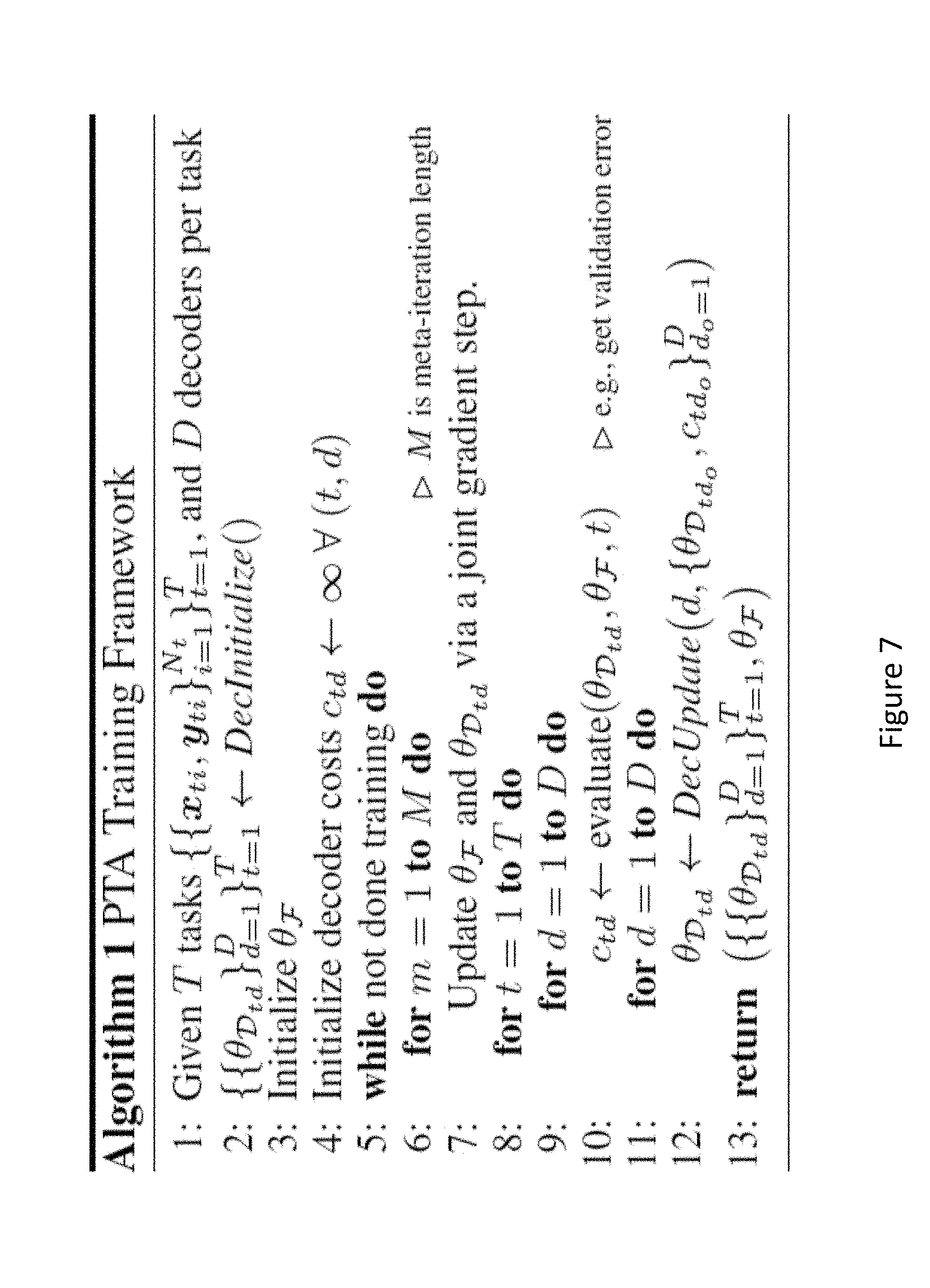
[0118] 1 D d = 1 D y ^ tdi = 1 D d = 1 D W td ( x ti ; .theta. ) W to = 1 D d = 1 D W td and .beta. = .alpha. . ##EQU00010## [0119] Knowing that training with additional pseudo-tasks yields augmented training dynamics, this may be exploited as discussed further herein. [0120] Given linear decoders, the primary goal is to optimize F; if an optimal F were found, optimal decoders for each task could be derived analytically. So, given multiple linear decoders for each task, how should their induced pseudotasks be controlled to maximize the benefit to F? For one, their weights {W.sub.td}.sub.d=1.sup.D must not all be equal, otherwise we would have W.sub.to=W.sub.t1 and .gamma.=Da in the proof of: there exist differentiable functions F and sets of pseudo-tasks of a single task that cannot be simulated by a single pseudo-task of that task, even when all decoders are linear Following Eq. 2, decoders can be trained jointly with F via gradient-based methods, so that they learn to work well with F. Through optimization, a trained decoder induces a trajectory of pseudo-tasks. Going beyond this implicit control, Algorithm 1 set forth in FIG. 7 gives a high-level framework for applying explicit control to pseudo-task trajectories. An instance of the algorithm is parameterized by choices for DecInitialize, which defines how decoders are initialized; and DecUpdate, which defines non-gradient-based updates to decoders every M gradient steps, i.e., every meta-iteration, based on the performance of each decoder (DecUpdate defaults to no-op). Several intuitive methods are evaluated for instantiating Algorithm 1. These methods can be used together in any combination.
[0121] First, the Independent Initialization (I) DecInitialize randomly initializes all .theta..sub.Dtd independently. This is the obvious initialization method, and is assumed in all methods below. Next, the Freeze (F) DecInitialize freezes all decoder weights except .theta..sub.Dt1 for each task. Frozen weights do not receive gradient updates in Line 7 of Algorithm 1. Because they cannot adapt to F, constant pseudo-task trajectories provide a stricter constraint on F. One decoder is left unfrozen so that the optimal model for each task can still be learned. The Independent Dropout (D) DecInitialize sets up the dropout layers preceding linear decoder layers to drop out values independently for each decoder. Thus, even when the weights of two decoders for a task are equal, their resulting gradient updates to F and to themselves will be different.
[0122] For the next three methods, let c.sub.t.sup.min=min(c.sub.t1, . . . , c.sub.tD), Perturb (P) DecUpdate adds noise.about.N(0, .sub.pI) to each .theta..sub.Dtd for all d where c.sub.td.noteq.c.sub.t.sup.min. This method ensures that .theta..sub.Dtd are sufficiently distinct before each training period. Hyperperturb (H) is like Perturb, except DecUpdate updates the hyperparameters of each decoder other than the best for each task, by adding noise.about.N(0, .sub.h). In these examples, each decoder has only one hyperparameter: the dropout rate of any Independent Dropout layer, because adapting dropout rates can be beneficial. Greedy (G) For each task, let .theta..sub.t.sup.min be the weights of a decoder with cost c.sub.t.sup.min. DecUpdate updates all .theta..sub.td:=.theta..sub.t.sup.min, including hyperparameters. This biases training to explore the highest-performing areas of the pseudo-task space. When combined with any of the previous three methods, decoder weights are still ensured to be distinct through training.
[0123] Combinations of these six methods induce an initial class of PTA training algorithms PTA-* for the case of linear decoders. The following eight representative combinations of these methods, i.e., PTA-I, PTA-F, PTA-P, PTA-D, PTA-FP, PTA-GP, PTA-GD, and PTA-HGD, in various experimental settings are evaluated below. Note that H and G are related to methods that copy the weights of the entire network. Also note that, in a possible future extension to the nonlinear case, the space of possible PTA control methods becomes much broader, as will be discussed herein.
Experiment
[0124] In this section, PTA methods are evaluated and shown to excel in a range of settings: (1) single-task character recognition; (2) multitask character recognition; (3) single-task sentiment classification; and (4) multitask visual attribute classification. All experiments are implemented using the Keras framework as is known in the art. For PTA-P and PTA-GP, .sub.p=0:01; for PTA-HGD, .sub.h=0:1 and dropout rates range from 0.2 to 0.8. A dropout layer with dropout rate initialized to 0.5 precedes each decoder.
Omniglot Character Recognition
[0125] The Omniglot dataset consists of 50 alphabets of handwritten characters, each of which induces its own character recognition task. Each character instance is a 105.times.105 black-and-white image, and each character has 20 instances, each drawn by a different individual. To reduce variance and improve reproducibility of experiments, a fixed random 50/20/30% train/validation/test split was used for each task. Methods are evaluated with respect to all 50 tasks as well as a subset consisting of the first 20 tasks in a fixed random ordering of alphabets used in previous work (Meyerson & Miikkulainen, Beyond Shared Hierarchies: Deep Multitask Learning through Soft Layer Ordering, ICLR (2018)). The underlying model F for all setups is a simple four layer convolutional network that has been shown to yield good performance on Omniglot. This model has four convolutional layers each with 53 filters and 3.times.3 kernels, and each followed by a 2.times.2 max-pooling layer and dropout layer with 0.5 dropout probability. At each meta-iteration, 250 gradient updates are performed via Adam; each setup is trained for 100 meta-iterations.
[0126] The single-task learning case is considered first. For each of the 20 initial Omniglot tasks, the eight PTA methods were applied to the task with 2, 3, and 4 decoders. At least three trials were run with each setup; the mean performance averaged across trials and tasks is shown in FIG. 8a. Every PTA setup outperforms the baseline, i.e., training with a single decoder. The methods that use decoder freezing, PTA-F and PTA-FP, perform best, showing how this problem can benefit from strong regularization. Notably, the mean improvement across all methods increases with D: 1.86% for D=2; 2.33% for D=3; and 2.70% for D=4. Like MTL can benefit from adding more tasks, single-task learning can benefit from adding more pseudo-tasks.
[0127] Omniglot models have also been shown to benefit from MTL. This section extends the experiments in STL to MTL. The setup is exactly the same, except now the underlying convolutional model is fully shared across all tasks for each method. The results are shown in FIG. 8b. All setups outperform the STL baseline, and all, except for PTA-I with D=2, outperform the MTL baseline. Again, PTA-F and PTA-FP perform best, and the mean improvement across all methods increases with D. The results show that although PTA implements behavior similar to MTL, when combined, their positive effects are complementary. Finally, to test the scalability of these results, three diverse PTA methods with D=4 and D=10 were applied to the complete 50-task dataset: PTA-I, because it is the baseline PTA method; PTA-F, because it is simple and high-performing; and PTA-HGD, because it is the most different from PTA-F, but also relatively high-performing. The results are given in Table 1.
TABLE-US-00001 TABLE 1 Method Single-task Multitask Learning Learning 35.49 29.02 Baseline D = 4 D = 10 D = 4 D = 10 PTA-I 31.72 32.56 27.26 24.50 PTA-HGD 31.63 30.39 25.77 26.55 PTA-F 29.37 28.48 23.45 23.36 PTA-Mean 30.91 30.48 25.49 24.80
The results agree with the 20-task results, with all methods improving upon the baseline, and performance overall improving as D is increased.
[0128] Next, PTA to LSTM models are applied in the IMDB sentiment classification problem. The dataset consists of 50K natural-language movie reviews, 25K for training and 25K for testing. There is a single binary classification task: whether a review is positive or negative. As in previous work, 2500 of the training reviews are withheld for validation. The underlying model F is the off-the-shelf LSTM model for IMDB provided by Keras, with no parameters or preprocessing changed. In particular, the vocabulary is capped at 20K words, the LSTM layer has 128 units and dropout rate 0.2, and each meta-iteration consists of one epoch of training with Adam. This model, but it is a very different architecture from that used in Omniglot, and therefore serves to demonstrate the broad applicability of PTA.
[0129] The final three PTA methods from Section 4.1 were evaluated with 4 and 10 decoders (Table 2).
TABLE-US-00002 TABLE 2 Method Test Accuracy % 82.75 (.+-.0.13) LSTM Baseline (D = 1) D = 4 D = 10 PTA-I 83.20 (.+-.0.07) 83.02 (.+-.0.11) PTA-HGD 83.22 (.+-.0.05) 83.51 (.+-.0.08) PTA-F 83.30 (.+-.0.12) 83.30 (.+-.0.08)
All PTA methods outperform the baseline. In this case, however, PTA-HGD with D=10 performs best. Notably, PTA-I and PTA-F do not improve from D=4 to D=10, suggesting that underlying models have a critical point after which, without careful control, too many decoders can be over constraining. To contrast PTA with standard regularization, additional Baseline experiments were run with dropout rates [0.3, 0.4, . . . , 0.9]. At 0.5 the best accuracy was achieved: 83.14 (+/-0.05), which is less than all PTA variants except PTA-I with D=10, thus confirming that PTA adds value. To help understand what each PTA method is actually doing, snapshots of decoder parameters taken every epoch are visualized in FIG. 9(a)-9(c) with t-SNE using cosine distance. Each shape corresponds to a particular decoder; each point is a projection of the length-129 weight vector at the end of an epoch, with opacity increasing by epoch. The behavior matches our intuition for what should be happening in each case: When decoders are only initialized independently, their pseudo-tasks gradually converge; when all but one decoder is frozen, the unfrozen one settles between the others; and when a greedy method is used, decoders perform local exploration as they traverse the pseudo-task space together.
[0130] To further test applicability and scalability, PTA was evaluated on CelebA large-scale facial attribute recognition. The dataset consists of .apprxeq.200K 178.times.218 color images. Each image has binary labels for 40 facial attributes; each attribute induces a binary classification task. Facial attributes are related at a high level that deep models can exploit, making CelebA a popular deep MTL benchmark. Thus, this experiment focuses on the MTL setting.
[0131] The underlying model was Inception-ResNet-v2, with weights initialized from training on ImageNet. Due to computational constraints, only one PTA method was evaluated: PTA-HGD with D=10. PTA-HGD was chosen because of its superior performance on IMDB, and because CelebA is a large-scale problem that may require extended pseudo-task exploration. FIG. 9(c) shows how PTA-HGD may support such exploration above other methods. Each meta-iteration consists of 250 gradient updates with batch size 32. The optimizer schedule is co-opted from previous work by Gunter et al., AFFACT--alignment free facial attribute classification technique. Corer, abs/1611.06158v2, 2017. RMSprop is initialized with a learning rate of 10.sup.-4, which is decreased to 10.sup.-5 and 10.sup.-6 when the model converges. PTA-HGD and the MTL baseline were each trained three times. The computational overhead of PTA-HGD is marginal, since the underlying model has 54M parameters, while each decoder has only 1.5K. Table 3 shows the results.
TABLE-US-00003 TABLE 3 MTL Method % Error Single Task (He et al., 2017) 10.37 MOON (Rudd et al., 2016) 9.06 Adaptive Sharing (Lu et al., 2017) 8.74 MCNN-AUX (Hand & Chellappa, 2017) 8.71 Soft Order (Meyerson & Miikkulainen, 2018) 8.64 VGG-16 MTL (Lu et al., 2017) 8.56 Adaptive Weighting (He et al., 2017) 8.20 AFFACT (Gunther et al., 2017) (best of 3) 8.16 MTL Baseline (Ours; mean of 3) 8.14 PTA-HGD, D = 10 (mean of 3) 8.10 Ensemble of 3: AFFACT (Gunther et al., 2017) 8.00 Ensemble of 3: PTA-HGD, D = 10 7.94
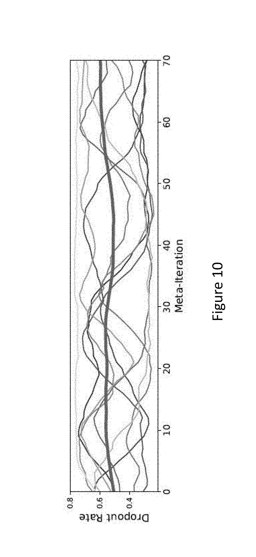
PTA-HGD outperforms all other methods, thus establishing a new state-of-the-art in CelebA. FIG. 10 shows resulting dropout schedules for PTA-HGD. The thick line shows the mean dropout schedule across all 400 pseudo-tasks in a run of PTA-HGD. Each of the remaining lines shows the schedule of a particular task, averaged across their 10 pseudo-tasks. All lines are plotted with a simple moving average of length 10. The diversity of schedules shows that the system is taking advantage of PTAHGD's ability to adapt task-specific hyperparameter schedules. No one type of schedule dominates; PTA-HGD gives each task the flexibility to adapt its own schedule via the performance of its pseudo-tasks.
[0132] As described herein PTA is broadly applicable, and can boost performance in a variety of single-task and multitask problems. Training with multiple decoders for a single task allows a broader set of models to be visited. If these decoders are diverse and perform well, then the shared structure has learned to solve the same problem in diverse ways, which is a hallmark of robust intelligence. In the MTL setting, controlling each task's pseudo-tasks independently makes it possible to discover diverse task-specific learning dynamics (FIG. 10). Increasing the number of decoders can also increase the chance that pairs of decoders align well across tasks. The crux of PTA is the method for controlling pseudo-task trajectories. Experiments showed that the amount of improvement from PTA is dependent on the choice of control method. Different methods exhibit highly structured but different behavior (FIGS. 9(a) to 9(c)). The success of initial methods indicates that developing more sophisticated methods is a promising avenue of future work. In particular, methods for training multiple models separately for a single task can be co-opted to control pseudo-task trajectories more effectively. Consider, for instance, the most involved method evaluated in this paper: PTA-HGD. This online decoder search method could be replaced by methods that generate new models more intelligently, such methods being known to those in the art. Such methods will be especially useful in extending PTA beyond the linear case considered in this paper, to complex nonlinear decoders. For example, since a set of decoders is being trained in parallel, it could be natural to use neural architecture search methods to search for optimal decoder architectures.
[0133] While the technology disclosed is disclosed by reference to various embodiments and examples detailed above, it is to be understood that these examples are intended in an illustrative rather than in a limiting sense. It is contemplated that modifications and combinations will readily occur to those skilled in the art, which modifications and combinations will be within the spirit of the innovation and the scope of the following claims.
* * * * *
D00000
D00001
D00002
D00003
D00004
D00005
D00006
D00007
D00008
D00009
D00010
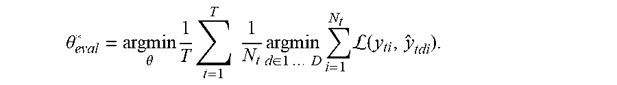
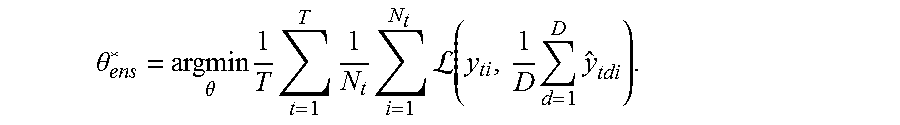
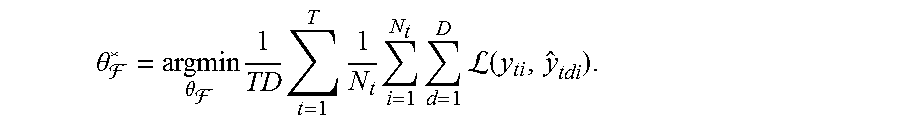
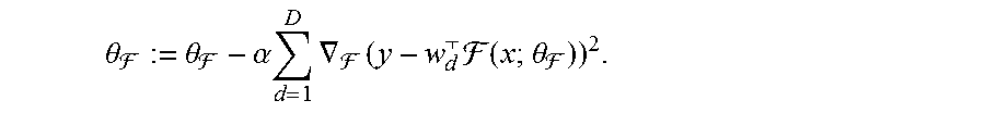
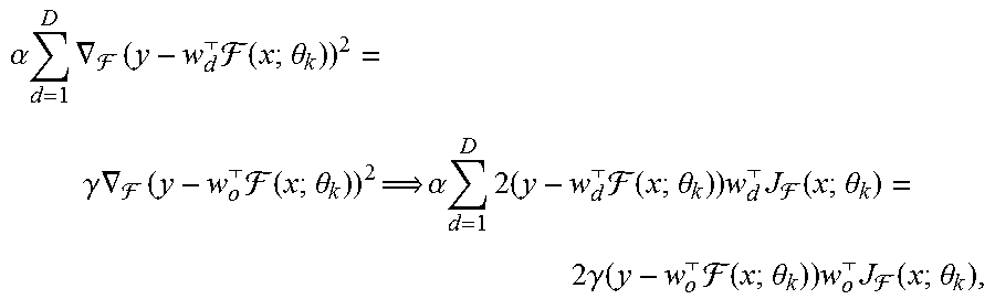
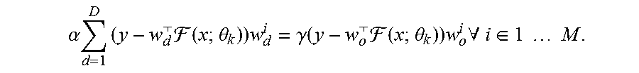
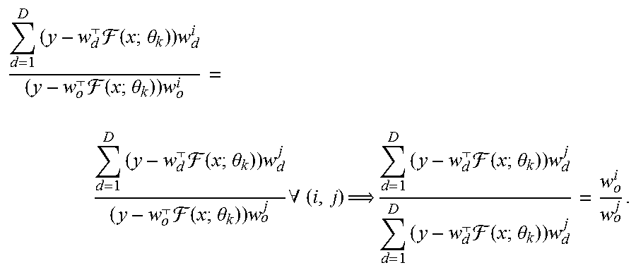
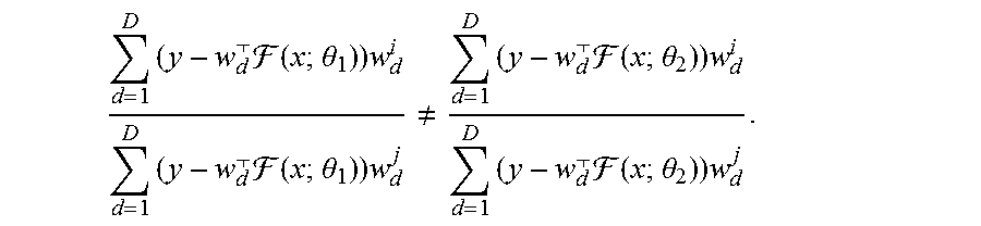
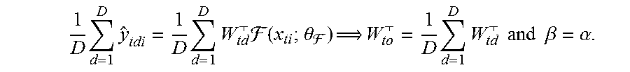
P00001

P00002

P00003

P00004

XML
uspto.report is an independent third-party trademark research tool that is not affiliated, endorsed, or sponsored by the United States Patent and Trademark Office (USPTO) or any other governmental organization. The information provided by uspto.report is based on publicly available data at the time of writing and is intended for informational purposes only.
While we strive to provide accurate and up-to-date information, we do not guarantee the accuracy, completeness, reliability, or suitability of the information displayed on this site. The use of this site is at your own risk. Any reliance you place on such information is therefore strictly at your own risk.
All official trademark data, including owner information, should be verified by visiting the official USPTO website at www.uspto.gov. This site is not intended to replace professional legal advice and should not be used as a substitute for consulting with a legal professional who is knowledgeable about trademark law.