A System And A Method For Determining A Trajectory To Be Followed By An Agricultural Work Vehicle
Green; Ole ; et al.
U.S. patent application number 16/338119 was filed with the patent office on 2019-08-08 for a system and a method for determining a trajectory to be followed by an agricultural work vehicle. The applicant listed for this patent is Agro Intelligence APS. Invention is credited to Gareth Thomas Charles Edwards, Ole Green.
| Application Number | 20190239416 16/338119 |
| Document ID | / |
| Family ID | 60051297 |
| Filed Date | 2019-08-08 |


View All Diagrams
| United States Patent Application | 20190239416 |
| Kind Code | A1 |
| Green; Ole ; et al. | August 8, 2019 |
A SYSTEM AND A METHOD FOR DETERMINING A TRAJECTORY TO BE FOLLOWED BY AN AGRICULTURAL WORK VEHICLE
Abstract
The present invention relates to a support system for determining a trajectory to be followed by an agricultural work vehicle, when working a field, said system comprises: a mapping unit configured for receiving: i) coordinates relating to the boundaries of a field to be worked; and ii) coordinates relating to the boundaries of one or more obstacles to be avoided by said work vehicle; wherein said one or more obstacles being located within said field; a capacity parameter unit configured for receiving one or more capacity parameters relating to said working vehicle; a trajectory calculating unit configured for calculating an optimized trajectory to be followed by said work vehicle; wherein said optimized trajectory is being calculated on the basis of said coordinates received by said mapping unit; and one or more of said one or more capacity parameters received by said capacity parameter unit.
| Inventors: | Green; Ole; (Lem, DK) ; Edwards; Gareth Thomas Charles; (Aarhus C, DK) | ||||||||||
| Applicant: |
|
||||||||||
|---|---|---|---|---|---|---|---|---|---|---|---|
| Family ID: | 60051297 | ||||||||||
| Appl. No.: | 16/338119 | ||||||||||
| Filed: | September 29, 2017 | ||||||||||
| PCT Filed: | September 29, 2017 | ||||||||||
| PCT NO: | PCT/DK2017/050321 | ||||||||||
| 371 Date: | March 29, 2019 |
| Current U.S. Class: | 1/1 |
| Current CPC Class: | A01B 69/007 20130101; G01C 21/20 20130101; G05D 2201/0201 20130101; A01B 69/008 20130101; G05D 1/0219 20130101; A01B 79/005 20130101 |
| International Class: | A01B 79/00 20060101 A01B079/00; G01C 21/20 20060101 G01C021/20; G05D 1/02 20060101 G05D001/02; A01B 69/04 20060101 A01B069/04 |
Foreign Application Data
| Date | Code | Application Number |
|---|---|---|
| Sep 29, 2016 | DK | PA 2016 00572 |
Claims
1. A support system for determining a trajectory to be followed by an agricultural work vehicle, when working a field, said system comprises: a mapping unit configured for receiving: i) coordinates relating to the boundaries of a field to be worked; and ii) coordinates relating to the boundaries of one or more obstacles to be avoided by said work vehicle; wherein said one or more obstacles being located within said field; a capacity parameter unit configured for receiving one or more capacity parameters relating to said working vehicle; a trajectory calculating unit configured for calculating an optimized trajectory to be followed by said work vehicle; wherein said optimized trajectory is being calculated on the basis of said coordinates received by said mapping unit; and one or more of said one or more capacity parameters received by said capacity parameter unit; wherein said trajectory calculating unit is being configured to perform the following steps: a) approximating the coordinates relating to the boundaries of said field to be worked to a boundary polygon; and wherein said support system is being configured to determine the trajectory to be followed, based on that approximation; b) approximating the coordinates relating to the boundaries of each said one or more obstacles, to respective obstacle polygons; and wherein said support system is being configured to determine the trajectory to be followed, based on that approximation; c) defining one or more headlands located immediately within said boundary polygon; d) in respect of each obstacle polygon, defining one or more headlands surrounding said obstacle polygon; e) defining a work area which corresponds to the area within said boundary polygon with the exclusion of the area corresponding to any headlands and with the exclusion of the area corresponding to any obstacle polygon; f) in respect of the orientation of one or more sides of headlands, define an array of parallel working rows located within said work area; g) in respect of one or more arrays of parallel working rows defined in step f), define an array of possible continuous driving paths by connecting separate entities, wherein said separate entities is being either headlands, or parts of a headland, and working rows, or parts of a working row; so as to define possible continuous driving paths, wherein each driving path is covering all headlands and all working rows; h) in respect of each of more possible continuous driving paths defined in step g), calculate an associated cost parameter, said calculated cost parameter being representative of the efficiency by following that specific continuous driving path; i) select as the trajectory to be followed, that specific continuous driving path exhibiting the highest efficiency . efficiency.
2-14. (canceled)
15. A method for determining a trajectory to be followed by an agricultural work vehicle, when working a field, said method comprising the steps: a) providing information relating to: i) coordinates relating to the boundaries of a field to be worked; and ii) coordinates relating to the boundaries of one or more obstacles to be avoided by said work vehicle; wherein said one or more obstacles being located within said field; b) providing information relating to: one or more capacity parameters relating to said working vehicle; c) performing a calculation of an optimized trajectory to be followed by said work vehicle; wherein said optimized trajectory is being calculated on the basis of said coordinates provided in step a) and b); wherein said method involves performing the following steps: a) approximating the coordinates relating to the boundaries of said field to be worked to a boundary polygon; b) approximating the coordinates relating to the boundaries of each said one or more obstacles, to respective obstacle polygons; c) defining one or more headlands located immediately within said boundary polygon; d) in respect of each obstacle polygon, defining one or more headlands surrounding said obstacle polygon; e) defining a work area which corresponds to the area within said boundary polygon with the exclusion of the area corresponding to any headlands and with the exclusion of the area corresponding to any obstacle polygon; f) in respect of the orientation of one or more sides of headlands, define an array of parallel working rows located within said work area; g) in respect of one or more arrays of parallel working rows defined in step f), define an array of possible continuous driving paths by connecting separate entities, wherein said separate entities is being either headlands, or parts of a headland, and working rows, or parts of a working row; so as to define possible continuous driving paths wherein each driving path is covering all headlands and all working rows; h) in respect of each of more possible continuous driving paths defined in step g), calculate an associated cost parameter, said calculated cost parameter being representative of the efficiency by following that specific continuous driving path; i) select as the trajectory to be followed, that specific continuous driving path exhibiting the highest efficiency.
16-28. (canceled)
29. A computer program product, which when loaded or operating on a computer, being adapted to perform the method according to claim 15.
30-32. (canceled)
Description
FIELD OF THE INVENTION
[0001] The present invention generally relates to the field of optimizing work trajectories of agricultural working vehicles for working a field. More specifically the present invention relates in a first aspect to a support system for determining a trajectory to be followed by an agricultural work vehicle when working a field. In a second aspect the present invention relates to a method for optimizing a trajectory to be followed by a work vehicle when working a field. In a third aspect the present invention relates to a computer program product which is adapted to perform the method according to the second aspect of the present invention. In a fourth aspect the present invention relates to an agricultural work vehicle comprising a support system according to the first aspect of the present invention. In a fifth aspect the present invention relates to a use of a support system according to the first aspect of the present invention, or of a computer program product according to the third aspect of the present invention, or of an agricultural work vehicle according to the fourth aspect of the present invention.
BACKGROUND OF THE INVENTION
[0002] Within the specific field of agriculture relating to growing crops, it has been known for thousands of years that in order to optimize crop yield the field has to be proper prepared and maintained. Accordingly, the field in which the crops are grown have to be prepared for seeding, then seeds have to be sown. During growth of the crops the field has to be fertilized and weeded and finally, when the crops have ripened, the crops are harvested.
[0003] All these preparation and maintenance operations, including harvesting will in a modern farming typically be performed using a motorized agricultural working vehicle, such as a tractor carrying or towing an implement, or the agricultural working vehicle may be self-propelled, such as it is know from harvesting machines.
[0004] Many fields used for growing crops are not free of obstacles. Accordingly, many fields used for growing crops will include a number of obstacles, such as creeks, ponds, clusters of trees, small hillocks, high voltage masts, electrical substations, wind turbines etc.
[0005] When working such fields comprising a number of obstacles these obstacles obviously have to be avoided by the working vehicle.
[0006] Most farmers when working a field comprising a number of obstacles simply follow a path based on habits. That is when working a field comprising a number of obstacles most farmers just follow the path that they use to follow when working that specific field, not paying particular attention to the question whether a more efficient path exist.
[0007] Furthermore, as various types of working implement for working a field will typically have different efficient working widths or other working parameters, it may not be the case that an optimum working path in respect of one working implement will be optimum in respect of another implement involving different working parameters.
[0008] Some agricultural working implement gain weight during operation, whereas others lose weight during operation thereof. Harvesters belong to the first category. Sowing machines and fertilizers belong to the second category.
[0009] As weight of the working vehicle, as a function of path travelled, may influence the immediate efficiency of the implement, also an optimized working trajectory may be dependent on the weight at a given position of the field. Accordingly, in order to optimize a working trajectory of an agricultural working implement, it may be necessary to take into consideration, the weight of the working implement at a given position on the trajectory.
[0010] When working farm land in a non-optimized way in which the trajectory which is followed is not an optimum trajectory, excessive time consumption in the working operation, excessive fuel consumption, excessive areas of the field covered more than once, and excessive wear on the working implement or machinery, or excessive travelling through the crops may result
[0011] Accordingly there is a persistent need for improving efficiency when working an agricultural field using a working vehicle.
[0012] It is an objective of the present invention to provide systems, uses and methods for improving efficiency when working an agricultural field using a working vehicle. Specifically it is an objective of the present invention to provide systems, uses and methods for determining an optimized trajectory to be followed by an agricultural work vehicle, when working an agricultural field.
BRIEF DESCRIPTION OF THE INVENTION
[0013] This objective is achieved by the present invention in its first, second, third, fourth and fifth aspect respectively.
[0014] Accordingly, in a first aspect, the present invention relates to a support system for determining a trajectory to be followed by an agricultural work vehicle, when working a field, said system comprises:
[0015] a mapping unit configured for receiving: [0016] i) coordinates relating to the boundaries of a field to be worked; and [0017] ii) coordinates relating to the boundaries of one or more obstacles to be avoided by said work vehicle; wherein said one or more obstacles being located within said field;
[0018] a capacity parameter unit configured for receiving one or more capacity parameters relating to said working vehicle;
[0019] a trajectory calculating unit configured for calculating an optimized trajectory to be followed by said work vehicle; wherein said optimized trajectory is being calculated on the basis of said coordinates received by said mapping unit; and one or more of said one or more capacity parameters received by said capacity parameter unit.
[0020] In a second aspect the present invention relates to a method for determining a trajectory to be followed by an agricultural work vehicle, when working a field, said method comprising the steps:
[0021] a) providing information relating to: [0022] i) coordinates relating to the boundaries of a field to be worked; and [0023] ii) coordinates relating to the boundaries of one or more obstacles to be avoided by said work vehicle; wherein said one or more obstacles being located within said field;
[0024] b) providing information relating to: [0025] one or more capacity parameters relating to said working vehicle;
[0026] c) performing a calculation of an optimized trajectory to be followed by said work vehicle; wherein said optimized trajectory is being calculated on the basis of said coordinates provided in step a) and b)
[0027] In a third aspect the present invention relates to a computer program product, which when loaded or operating on a computer, being adapted to perform the method according the second aspect.
[0028] In a fourth aspect the present invention relates to an agricultural work vehicle comprising a support system according to the first aspect.
[0029] In a fifth aspect the present invention relates to the use of a support system according to the first aspect of the present invention or of a computer program product according to the third aspect of the present invention or of an agricultural work vehicle according to the fourth aspect of the present invention for optimizing a trajectory to be followed by a work vehicle when working a field.
[0030] The present invention in its various aspects provides for optimizing a path to be followed by a working vehicle or a working implement upon working a field. Thereby a high working efficiency is obtained. The efficiency may relate to saving time, saving fuel, saving wear and tear of the machinery employed, minimizing total distance travelled twice or more, minimizing total area covered twice etc.
BRIEF DESCRIPTION OF THE FIGURES
[0031] FIG. 1 is a top view of a field comprising a number of obstacles located within its boundary and illustrates the problems associated with working such a field.
[0032] FIG. 2 is a diagrammatic illustration of the working mode of a support system according to the present invention.
[0033] FIG. 3-23d are illustrations relating to Example 1 illustrates how to mathematically manage to create possible continuous driving paths in an agricultural field and how to find an optimum driving path amongst those possible continuous driving paths.
[0034] FIG. 24-29 illustrates the individual steps associated with performing one embodiment of the method according to the present invention.
[0035] FIG. 30 is a flow diagram illustrating an iterative procedure for use in one embodiment of the method according to the present invention.
DETAILED DESCRIPTION OF THE INVENTION
[0036] In a first aspect the present invention relates to a support system for determining a trajectory to be followed by an agricultural work vehicle, when working a field, said system comprises:
[0037] a mapping unit configured for receiving: [0038] i) coordinates relating to the boundaries of a field to be worked; and [0039] ii) coordinates relating to the boundaries of one or more obstacles to be avoided by said work vehicle; wherein said one or more obstacles being located within said field;
[0040] a capacity parameter unit configured for receiving one or more capacity parameters relating to said working vehicle;
[0041] a trajectory calculating unit configured for calculating an optimized trajectory to be followed by said work vehicle; wherein said optimized trajectory is being calculated on the basis of said coordinates received by said mapping unit; and one or more of said one or more capacity parameters received by said capacity parameter unit.
[0042] The support system is designed with the view to aid in optimizing finding a trajectory to be followed upon working an agricultural field with a working vehicle or implement.
[0043] The support system may be in the form of electronic equipment configured for receiving inputs relating to coordinates of the field and obstacles therein. The support system is further configured to using these inputted inputs to determine an optimized trajectory to be followed. The support system typically makes use of a computer for performing calculations, such as iterative calculations.
[0044] The various units may independently be connected to each other, or at least be able to communicate with each other. The support system may comprise separate entities or be integrated.
[0045] In one embodiment of the first aspect of the present invention said mapping unit is furthermore is configured for receiving: [0046] iii) coordinates relating to the possible entrance/exit gates of the field.
[0047] This ensures that the position or positions of entrance/exit gates are taking into consideration when calculating the optimized trajectory to be followed.
[0048] In one embodiment of the first aspect of the present invention said optimized trajectory is being an optimized trajectory in terms of total operational time for working the field; total productive time for working the field; total fuel consumption for working the field; total non-working distance for working the field; total distance travelled twice or more; total distance travelled through crops; total area covered twice or more.
[0049] Depending on which concern after which the trajectory is to be optimized, a number of different optimizations parameters are possible. Above, a few of these are listed.
[0050] In one embodiment of the first aspect of the present invention said one or more capacity parameters is being selected from the group comprising: effective working width of the work vehicle or the working implement, load of work vehicle as a function of distance travelled, fuel consumption as a function of distance travelled, minimum turning radius of vehicle or implement or both.
[0051] These parameters are parameters which may be relevant in finding an optimized trajectory to follow when working a field.
[0052] In one embodiment of the first aspect of the present invention said support system further comprising a display unit configured to be able to show on a map of said filed, the optimized trajectory to be followed by said work vehicle as calculated by said trajectory calculating unit.
[0053] This will enable the driver of the working vehicle or implement to easily follow the optimized trajectory, once this has been provided by the trajectory calculating unit.
[0054] In one embodiment of the first aspect of the present invention said mapping unit is being configured for storing, in respect of one or more specific fields, one or more of: i) coordinates relating to the boundaries of said one or more specific fields; ii) coordinates relating to the boundaries of one or more obstacles being located within said one or more specific fields; and iii) coordinates relating to the possible entrance/exit gates of said one or more specific fields.
[0055] This will allow minimizing the amount of input needed from time to time.
[0056] In one embodiment of the first aspect of the present invention said trajectory calculating unit is configured to calculate an optimized trajectory analytically or numerically.
[0057] Analytically or numerically calculation strategies are two strategies that are particularly well suited in respect of the present invention.
[0058] In one embodiment of the first aspect of the present invention said trajectory calculating unit is being configured to find a number of candidate trajectories, and wherein said trajectory calculating unit is configured to calculate, in respect of each candidate trajectory, an efficiency parameter, and wherein said trajectory calculating unit is configured to suggest to the user, that specific candidate trajectory, which exhibits the highest efficiency parameter.
[0059] Such a mode of operation of the support system is particularly preferred.
[0060] In one embodiment of the first aspect of the present invention said trajectory calculating unit is being configured to perform the following steps: [0061] a) approximating the coordinates relating to the boundaries of said field to be worked to a boundary polygon; and wherein said support system is being configured to determine the trajectory to be followed, based on that approximation; [0062] b) approximating the coordinates relating to the boundaries of each said one or more obstacles, to respective obstacle polygons; and wherein said support system is being configured to determine the trajectory to be followed, based on that approximation; [0063] c) defining one or more headlands located immediately within said boundary polygon; [0064] d) in respect of each obstacle polygon, defining one or more headlands surrounding said obstacle polygon; [0065] e) defining a work area which corresponds to the area within said boundary polygon with the exclusion of the area corresponding to any headlands and with the exclusion of the area corresponding to any obstacle polygon; [0066] f) in respect of the orientation of one or more sides of headlands, define an array of parallel working rows located within said work area; [0067] g) in respect of one or more arrays of parallel working rows defined in step f), define an array of possible continuous driving paths by connecting separate entities, wherein said separate entities is being either headlands, or parts of a headland, and working rows, or parts of a working row; so as to define possible continuous driving paths, wherein each driving path is covering all headlands and all working rows; [0068] h) in respect of each of more possible continuous driving paths defined in step g), calculate an associated cost parameter, said calculated cost parameter being representative of the efficiency by following that specific continuous driving path; [0069] i) select as the trajectory to be followed, that specific continuous driving path exhibiting the highest efficiency.
[0070] Hereby it is possible in a clever and well-organized way to allow the trajectory calculating unit to find an optimized trajectory to be followed.
[0071] In one embodiment of the first aspect of the present invention said trajectory calculating unit is being configured to create a possible continuous path by first choosing a particular entrance/exit gate.
[0072] As the entrance/exit gate(s) is/are fixed constraint(s) it has proven beneficial to operate the system this way.
[0073] In one embodiment of the first aspect of the present invention said headland surrounding said obstacle polygon in respect of one or more of said obstacle polygons, includes a safety offset area surrounding said obstacle polygon.
[0074] Including a safety offset area surrounding said obstacle polygon will enhance safety when operating the work vehicle or implement as collision hazards will be reduced this way.
[0075] In one embodiment of the first aspect of the present invention each said working row and/or each said headland independently are having a width corresponding to the effective working width of the work vehicle or working implement.
[0076] It is beneficial to create working paths having widths corresponding to the effective working width of the work vehicle or working implement.
[0077] In one embodiment of the first aspect of the present invention said support system being configured for defining a number of possible continues driven paths, each comprising a sequence of straight line segments and arched line segments.
[0078] Hereby it will be possible for the driver of the work vehicle or implement to follow one continuous path.
[0079] In one embodiment of the first aspect of the present invention said support system is being configured to find said optimized trajectory by means of a heuristic method, such as a greedy heuristic method, a tabu search solver, an ant colony solver, a genetic algorithm.
[0080] Such heuristic method will reduce the amount of data processing necessary for the trajectory calculating unit.
[0081] In one embodiment of the first aspect of the present invention said support system is being configured to create a number N of possible continuous driven paths with an associated assigned cost parameter, and wherein said number N being an integer in the range 1,000-700,000 or more, for example 2,000-600,000, such as 5,000-500,000, e.g. 10,000-400,000, such as 50,000-300,000 or 100,000-200,000 possible continuous driven paths with an associated assigned cost parameter.
[0082] Such numbers of choices to choose from will enhance the reliability of the trajectory found by the system.
[0083] In a second aspect the present invention relates to a method for determining a trajectory to be followed by an agricultural work vehicle, when working a field, said method comprising the steps:
[0084] a) providing information relating to: [0085] i) coordinates relating to the boundaries of a field to be worked; and [0086] ii) coordinates relating to the boundaries of one or more obstacles to be avoided by said work vehicle; wherein said one or more obstacles being located within said field;
[0087] b) providing information relating to: [0088] one or more capacity parameters relating to said working vehicle;
[0089] c) performing a calculation of an optimized trajectory to be followed by said work vehicle; wherein said optimized trajectory is being calculated on the basis of said coordinates provided in step a) and b)
[0090] In one embodiment of the second aspect of the present invention said step a) furthermore is involves providing [0091] iii) coordinates relating to the possible entrance/exit gates of the field.
[0092] This ensures that the position or positions of entrance/exit gates are taking into consideration when calculating the optimized trajectory to be followed.
[0093] In one embodiment of the second aspect of the present invention said optimized trajectory is an optimized trajectory in terms of total operational time for working the field; total productive time for working the field; total fuel consumption for working the field; total non-working distance for working the field; total distance travelled twice or more; total distance travelled through crops; total area covered twice or more.
[0094] Depending on which concern after which the trajectory is to be optimized, a number of different optimizations parameters are possible. Above, a few of these are listed.
[0095] In one embodiment of the second aspect of the present invention said one or more capacity parameters being selected from the group comprising: effective working width of the work vehicle or the working implement, load of work vehicle as a function of distance travelled, fuel consumption as a function of distance travelled, minimum turning radius of vehicle or implement or both.
[0096] These parameters are parameters which may be relevant in finding an optimized trajectory to follow when working a field.
[0097] In one embodiment of the second aspect of the present invention said optimized trajectory to be followed by said work vehicle is being presented in a graphical presentation such as being showed on an electronic map of said field to be worked.
[0098] This will enable the driver of the working vehicle or implement to easily follow the optimized trajectory, once this has been provided by the trajectory calculating unit.
[0099] In one embodiment of the second aspect of the present invention said method involving calculation of said optimized trajectory analytically or numerically.
[0100] Analytically or numerically calculation strategies are two strategies that are particularly well suited in respect of the present invention.
[0101] In one embodiment of the second aspect of the present invention said method involves finding a number of candidate trajectories; calculation in respect of each candidate trajectory, an efficiency parameter; and suggesting to a user, that specific candidate trajectory, which exhibits the highest efficiency parameter.
[0102] Such a mode of operation of the method is particularly preferred.
[0103] In one embodiment of the second aspect of the present invention said method involves performing the following steps: [0104] a) approximating the coordinates relating to the boundaries of said field to be worked to a boundary polygon; [0105] b) approximating the coordinates relating to the boundaries of each said one or more obstacles, to respective obstacle polygons; [0106] c) defining one or more headlands located immediately within said boundary polygon; [0107] d) in respect of each obstacle polygon, defining one or more headlands surrounding said obstacle polygon; [0108] e) defining a work area which corresponds to the area within said boundary polygon with the exclusion of the area corresponding to any headlands and with the exclusion of the area corresponding to any obstacle polygon; [0109] f) in respect of the orientation of one or more sides of headlands, define an array of parallel working rows located within said work area; [0110] g) in respect of one or more arrays of parallel working rows defined in step 0, define an array of possible continuous driving paths by connecting separate entities, wherein said separate entities is being either headlands, or parts of a headland, and working rows, or parts of a working row; so as to define possible continuous driving paths wherein each driving path is covering all headlands and all working rows; [0111] h) in respect of each of more possible continuous driving paths defined in step g), calculate an associated cost parameter, said calculated cost parameter being representative of the efficiency by following that specific continuous driving path; [0112] i) select as the trajectory to be followed, that specific continuous driving path exhibiting the highest efficiency.
[0113] Hereby it is possible in a clever and well-organized way to calculate and find an optimized trajectory to be followed.
[0114] In one embodiment of the second aspect of the present invention said method involves creation of a possible continuous path by first choosing a particular entrance/exit gate.
[0115] As the entrance/exit gate(s) is/are fixed constraint it has proven beneficial to operate the method this way.
[0116] In one embodiment of the second aspect of the present invention said headland surrounding said obstacle polygon, in respect of one or more of said obstacle polygons, includes a safety offset area surrounding said obstacle polygon.
[0117] Including a safety offset area surrounding said obstacle polygon will enhance safety when operating the work vehicle or implement as collision hazards will be reduced this way.
[0118] In one embodiment of the second aspect of the present invention each said working row and/or each said headland independently are having a width corresponding to the effective working width of the work vehicle or working implement.
[0119] It is beneficial to create working paths having widths corresponding to the effective working width of the work vehicle or working implement.
[0120] In one embodiment of the second aspect of the present invention said method involves defining a number of possible continuous driven paths, each comprising a sequence of straight line segments and arched line segments.
[0121] In one embodiment of the second aspect of the present invention said method involves finding said optimized trajectory by means of a heuristic method, such as a greedy heuristic method, a tabu search solver, an ant colony solver, a genetic algorithm.
[0122] Such heuristic method will reduce the amount of data processing necessary involved in the method.
[0123] In one embodiment of the second aspect of the present invention said method involves creating a number N of possible continuous driven paths with an associated assigned cost parameter, and wherein said number N being an integer in the range 1,000-700,000, possible continuous driven paths with an associated assigned cost parameter, such as 5,000-500,000, e.g. 10,000-400,000, such as 50,000-300,000 or 100,000-200,000 possible continuous driven paths with an associated assigned cost parameter.
[0124] Such numbers of choices to choose from will enhance the reliability of the trajectory found in the method.
[0125] In one embodiment of the second aspect of the present invention said method being performed by using a support system according to the first aspect of the present invention.
[0126] In a third aspect the present invention relates to a computer program product, which when loaded or operating on a computer, being adapted to perform the method according to the second aspect of the present invention.
[0127] In the present description and in the appended claims it shall be understood that a computer program product may be presented in the form of a piece of software which is storable or stored on a piece of hardware. Hereby, the computer program product may be embodied in one or more computer readable storage media as a computer readable program code embodied thereon.
[0128] Accordingly, the computer program product may be presented as a computer-readable storage medium having a computer program product embodied therein.
[0129] The computer program code is configured for carrying out the operations of the method according to the first aspect of the present invention and it may be written in any combination of one or more programming languages.
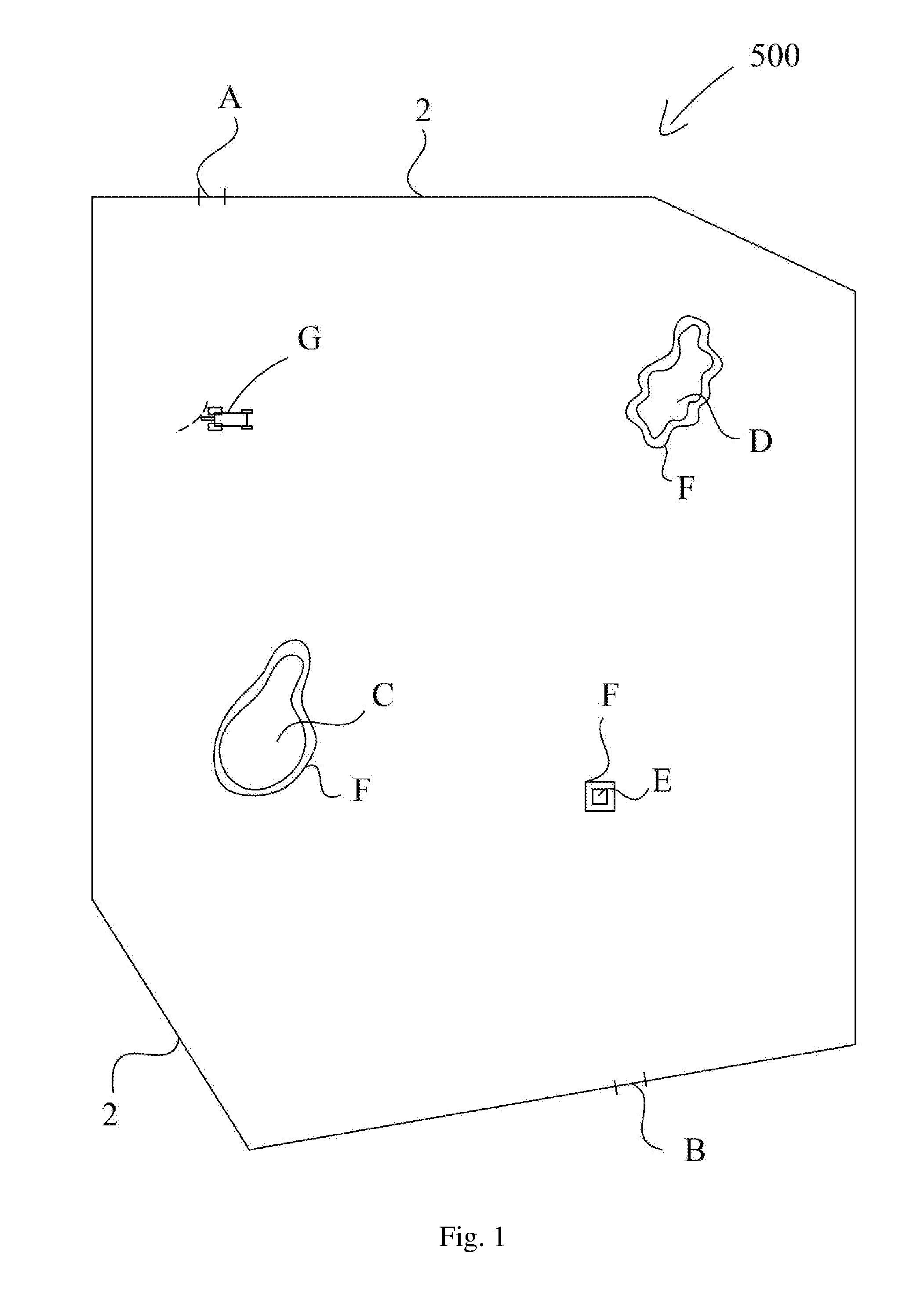
[0130] In a fourth aspect the present invention relates to an agricultural work vehicle comprising a support system according to the first aspect of the present invention.
[0131] In a fifth aspect the present invention relates to the use of a support system according to the first aspect of the present invention, or of a computer program product according to the third aspect of the present invention, of an agricultural work vehicle according to the fourth aspect of the present invention. for optimizing a trajectory to be followed by said work vehicle when working a field.
[0132] In the present description and in the appended claims the following definitions shall be adhered to:
[0133] Field to be worked: A field to be worked shall be understood to comprise a limited area of a field which content or surface need to be subjected to an agricultural activity.
[0134] Obstacle: An obstacle shall be understood to comprise a physical entity which is located within or which has an extension which extends into a field to be worked and which presence prevents working the field at the location of that obstacle.
[0135] Boundary polygon: A boundary polygon shall be understood to be a polygon which has a size and a shape which approximates the boundary of a field to be worked.
[0136] Obstacle polygon: An obstacle polygon shall be understood to be a polygon which has a size and a shape which approximates the boundary of an obstacle.
[0137] Headland: A headland shall be understood to be an area located immediately within the boundary of a field to be worked, or within a boundary polygon; or which surrounds an obstacle in close proximity thereof.
[0138] Mainland: A mainland shall be understood to be an area located within a field boundary or within a boundary polygon, excluding any area corresponding to headlands.
[0139] Safety offset area: A safety offset area is an area surrounding an obstacle, or an obstacle polygon, thereby rendering the effective size of an obstacle greater that the obstacle, or obstacle polygon itself. A safety offset area serves the purpose of creating a safety distance from an obstacle to a working vehicle or implement in order to avoid collision with that obstacle.
[0140] Work area: A work area shall be understood to mean the area comprised inside the boundary of a field to be worked, or an approximation thereof, and excluding any headland; and excluding any obstacles, or approximation of any obstacles including a safety offset area of one or more obstacles.
[0141] Working row: A working row shall be understood to mean a row located within a work area and which preferably is having a width corresponding to the effective working width of the soil working vehicle or implement.
[0142] Cost parameter: A cost parameter shall be understood to mean a parameter expressing a relative efficiency in following a specific path.
[0143] Optimized trajectory: An optimized trajectory shall be understood to mean that trajectory which, compared to other trajectories under investigation, is most efficient in terms of a cost parameter. An optimized trajectory needs may or may not be a globally optimized trajectory. In some instances an optimized trajectory merely expresses an intelligent and qualified suggestion for a best path to follow when working a field.
[0144] Now referring to the figures for the purpose of illustration the present invention, FIG. 1 shows an overhead plan view of a field 500 to be worked by an agricultural working vehicle or implement. The field comprises two possible entrances/exits A and B located at the boundary 2 of the field. Within the field a number of obstacles are present. These obstacles must be avoided when working the field. The obstacles being present in the field 500 shown in FIG. 1 include a pond C, a cluster of trees D and a high voltage mast E. Each of the obstacles is surrounded by a safety margin F. The safety margin serves the purpose of not getting too close to the obstacles when working the field, and is thereby intended for avoiding any hazardous situation relating to impact between the working vehicle and the obstacles.
[0145] Also illustrated in FIG. 1 is a working vehicle G in the form of a tractor towing a plough.
[0146] It is easily acknowledged that the field 500 with its obstacles C, D and E and its entrances/exits A and B illustrated in FIG. 1 allows for an almost indefinitely number of possible trajectories for working the whole field, and that the human brain is not in itself without any technological aid capable to immediately tell which working path or working trajectory will be most efficient.
[0147] FIG. 2 is a diagram which illustrates the working mode of one embodiment of the support system for determining a trajectory to be followed by an agricultural work vehicle according to the first aspect of the present invention.
[0148] FIG. 2 shows the support system 100 for determining a trajectory to be followed by an agricultural work vehicle. The support system comprises a mapping unit MU configured for receiving information I.sub.1 in the form of coordinates relating to the boundaries of a field to be worked; and information I.sub.2 in the form of coordinates relating to the boundaries of one or more obstacles within said field and to be avoided by said work vehicle; and information I.sub.3 in the form of coordinates relating to the possible entrance(s)/exit(s) of a specific field to be worked.
[0149] The support system further comprises a capacity parameter unit CU configured for receiving information I.sub.4 relating to one or more capacity parameters relating to said working vehicle.
[0150] The one or more capacity parameters may relate to effective working width of the work vehicle or the working implement, load of work vehicle as a function of distance travelled, fuel consumption as a function of distance travelled, truning radius of the work vehicle etc.
[0151] Based on the information I.sub.1, I.sub.2 and I.sub.3 provided to said mapping unit MU and based on the information I.sub.4 provided to said capacity parameter unit CU, a trajectory calculating unit TCU is calculating an optimized trajectory to be followed by said work vehicle. The calculated optimized work trajectory is displayed on the display M which also outlines the field itself
[0152] The calculation may be an analytical calculation or a numerical calculation.
EXAMPLES
[0153] The following example illustrates on embodiment of various aspects of the present invention.
Example 1
[0154] The following example discloses in detail one way of performing the mathematical operations necessary in the process of going from a field boundary to creating possible individual candidate trajectories and the step of assigning an efficiency parameter to each of those candidate trajectories so that the most efficient candidate trajectory can be chosen as the optimum trajectory when working that field with an agricultural working vehicle or implement.
[0155] The present example is based on the principle involving the following steps: [0156] a) approximating the coordinates relating to the boundaries of said field to be worked to a boundary polygon; [0157] b) approximating the coordinates relating to the boundaries of each said one or more obstacles, to respective obstacle polygons; [0158] c) defining one or more headlands located immediately within said boundary polygon; [0159] d) in respect of each obstacle polygon, defining one or more headlands surrounding said obstacle polygon; [0160] e) defining a work area which corresponds to the area within said boundary polygon with the exclusion of the area corresponding to any headlands and with the exclusion of the area corresponding to any obstacle polygon; [0161] f) in respect of the orientation of one or more sides of headlands, define an array of parallel working rows located within said work area; [0162] g) in respect of one or more arrays of parallel working rows defined in step f), define an array of possible continuous driving paths by connecting separate entities, wherein said separate entities is being either headlands, or parts of a headland, and working rows, or parts of a working row; so as to define possible continuous driving paths, wherein each driving path is covering all headlands and all working rows; [0163] h) in respect of each of more possible continuous driving paths defined in step g), calculate an associated cost parameter, said calculated cost parameter being representative of the efficiency by following that specific continuous driving path; [0164] i) select as the trajectory to be followed, that specific continuous driving path exhibiting the highest efficiency.
[0165] Other principles may equally well work with the present invention in its various aspects.
[0166] In the calculation of the present example the following inputs are needed. [0167] Defined Field Boundary [0168] Defined Obstacle Boundary [0169] Defined Field Gates [0170] Vehicle working width [0171] Vehicle turning radius [0172] Specified number of headlands
[0173] Processing Steps
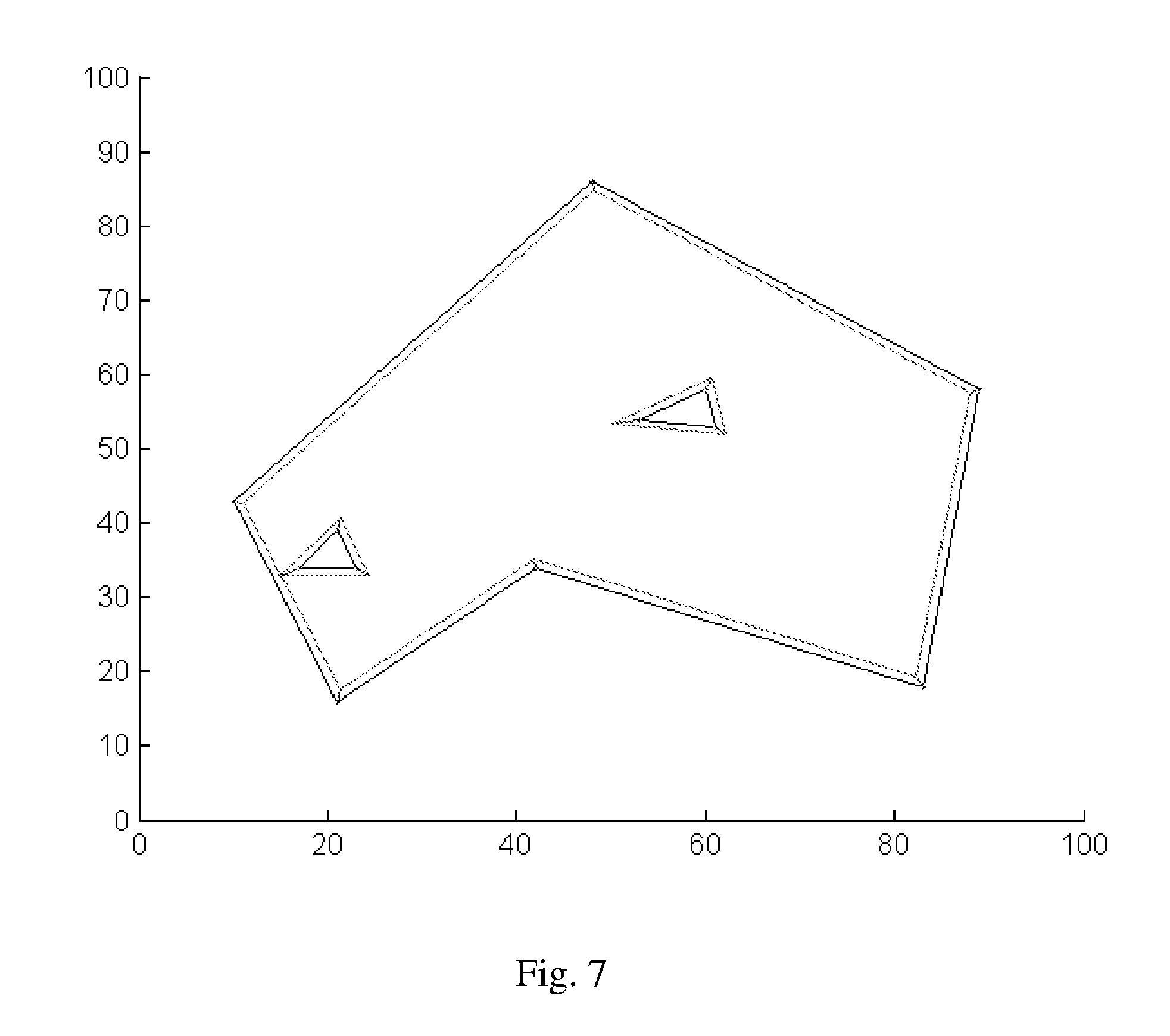
[0174] Field Definition
[0175] The field is described by the field boundary which is a polygon consisting of n points. In FIG. 3 the polygon P consists of 6 point (P.sub.1, . . . ,P.sub.6). The points of P are ordered such that they are in a clockwise orientation. P=([10,43],[48,86],[89,58],[83,18],[42,34],[21,16]). See FIG. 3.
[0176] Within the boundary there are a number of obstacles. The obstacles the obstacles are described by a boundary. This may be the physical edge of the obstacle or it may also include a "safety offset" to ensure working vehicles remain a safe distance away. In FIG. 4 the obstacles are described as polygons (O.sup.1, O.sup.2) with points (O.sup.1.sub.1, . . . , O.sup.1.sub.3) and (O.sup.2.sub.1, . . . , O.sup.2.sub.3). The points of the obstacles are ordered such they are in an anti-clockwise orientation. O.sup.1=([23,34],[21,39],[17,34]), and O.sup.2=([60,58],[53,54],[61,53]). See FIG. 4
[0177] A number of gates are defined for the field. These are entry/exit point for the field and are located on the field boundary. In this example there is one gate G.sup.1[83,18].
[0178] The working width is the effective working width of the agricultural machine or implement. The turning radius is minimum radius the vehicle can turn. For a standard two axle vehicle with one axle steering it can be calculated by dividing the distance between the front and rear axles of the vehicle by the tangent of the maximum angle of the steering axle.
[0179] Creating the Headlands
[0180] The headlands are areas which encompass the field boundary and the surround the obstacle. These areas are used by the vehicle to more easily manoeuvre in the field. The number of headlands required to safely operate in a field is the integer greater than 2*turning radius divided working width. The headlands have an outer boundary and an inner boundary. For the first headland areas the outer boundary is the boundary of the field or the obstacle and the inner boundary plotted such that the area between the outer boundary and inner boundary has a width equal to the working width. For subsequent headlands, the outer boundary is the inner boundary of the previous headland.
[0181] To calculate the headland areas the boundary of the field and the boundary of each obstacle are expressed as a set consisting of 3 arrays {P, V, A}, where P is the array of corner points of the boundary, V is the array of vertices linking the corners of the boundary and A is the array of vectors at the apex of each boundary point.
V i = P i + 1 - P i : i = 1 p - 1 ##EQU00001## V p = P 1 - P p ##EQU00001.2## A i - V i - 1 A i V i - 1 = cos .theta. = A i V i A i V i , A i [ V i , y - V i , x ] A i V i < A i [ - V i , y V i , x ] A i V i ##EQU00001.3## A i = 1 sin .theta. ##EQU00001.4##
[0182] This is illustrated in FIG. 5.
[0183] The constrain on A.sub.i ensures that the A.sub.i vector always points to the right of the V.sub.i vector. See FIG. 5,
[0184] In FIG. 6 the P, V, and A arrays are labelled for the field boundary. In the example for the field boundary V=([38,43],[41,-28],[-6,-40],[-41,16],[-21,-18],[-11,27]) and A=([1.16,-0.20],[0.16,-1.32], [-1.08,-0.47],[-0.80,1.39], [-0.2,1.15],[0.40,1.66]).
[0185] To create the inner boundary, the corners of the outer boundary are projected along the apex vector, so that they maintain an equal perpendicular distance from the two vectors creating the corner. Therefore for a distance .lamda. a new boundary can be created as a new set of point P'.
P'.sub.i=P.sub.i+.lamda.*A.sub.i: i=1, . . . , p
[0186] V' and A' can then be created using the above equations.
[0187] There are 3 cases which must be monitored when creating the new boundary. The 3 cases are a self-corner interception, a self-edge interception and a 2 polygon interception.
[0188] Case 1:
[0189] The self-corner interception occurs when two adjacent apex vectors intersect, resulting in V' to have a zero length and P.sub.i=P.sub.i+1. Therefore for each P there is a value, .alpha., where this happens.
P i ' = P i + .alpha. i * A i = P i + 1 + .alpha. i * A i + 1 = P i + 1 ' : i = 1 p - 1 ##EQU00002## P 1 ' = P 1 + .alpha. p * A 1 = P p + .alpha. p * A p = P p ' ##EQU00002.2## .alpha. i = P i + 1 - P A i - A i + 1 : i = 1 p - 1 ##EQU00002.3## .alpha. p = P 1 - P p A p - A 1 ##EQU00002.4## .alpha. n = min { .alpha. i } : .alpha. i > 0 , i = 1 p ##EQU00002.5##
[0190] If a self-corner interception occurs P'.sub.i is removed from P', and V' and A' are recalculated.
[0191] For the example of the field boundary the .alpha.=[38.34,36.76,40.9,36.89,160.54,14.89]. Therefore .alpha..sub.n=14.89. Since O1 and O2 are both triangles with the points arrange in an anti-clockwise orientation it is impossible a self-corner interception to occur.
[0192] Case 2:
[0193] The self-edge interception occurs when an apex vector intersects a vertex between two points.
P'.sub.i=P'.sub.j+b*V'.sub.j: i,j=1, . . . p; i.noteq.j, 0<b<1
[0194] Therefore for each pair of point P.sub.i and P.sub.j there is a value, .beta..sub.i,j, where this occurs.
.beta. ij = P j + 1 - P j - P i A i + A j - A j + 1 : i = 1 p , j = 1 p - 1 , i .noteq. j , i .noteq. j + 1 ##EQU00003## .beta. ip = P 1 - P p - P i A i + A p - A 1 : i = 1 p - 1 ##EQU00003.2## .beta. n m = min { min { .beta. ij } j } i : i = 1 p , j = 1 p , .beta. ij > 0 ##EQU00003.3##
[0195] If a self-edge interaction occurs then P' is split into two subsets, .sup.1P' and .sup.2P' and V' and A' are recalculated.
P'.sub.i=P.sub.i+.beta..sub.nm*A.sub.i: i=1 . . . p
.sup.1P'={P'.sub.1, . . . , P'.sub.n, P'.sub.m+1, . . . , P'.sub.p}, .sup.2P'={P'.sub.n, . . . , P'.sub.m} if n<m
.sup.1P'={P'.sub.1, . . . , P'.sub.m, P'.sub.n, . . . , P'.sub.p}, .sup.2P'={P'.sub.m+1, . . . , P'.sub.n} if n>m
[0196] For the example field .beta..sub.ij is describing in the Table 1 below.
TABLE-US-00001 TABLE 1 j\i 1 2 3 4 5 6 1 -- 38.24 32.79 -4.22 16.76 -- 2 -- -- 29.96 23.26 19.23 38.18 3 23.21 -- -- 41.13 39.04 43.31 4 28.25 21.46 -- -- 46.61 47.95 5 18.55 22.46 36.84 -- -- 69.48 6 14.50 28.13 47.40 35.48 -- --
[0197] Therefore .beta..sub.nm=14.50, n=1, m=6. Again since O1 and O2 are both triangles and therefore only have 3 points it is impossible a self-edge interception to occur.
[0198] Case 3:
[0199] The 2 polygon interception occurs when two polygon sets, such as a field boundary and an obstacle boundary intercept. NB if two polygons are created due to case 2 these two polygon it is impossible that these two polygons can intercept.
.gamma. ij gh = P j h - P j + 1 h - P i g A i g + A j h - A j + 1 h : i = 1 g p , j = 1 h p - 1 , g , h = 1 , N , g .noteq. h ##EQU00004##
[0200] Where N, is the number of active sets describing polygons.
.gamma. n m kl = min { min { min { min { .gamma. ij gh } j } i } h } g ##EQU00005##
[0201] If a 2 polygon interception occurs the two polygons become merged together to form a new polygon, with the original two polygons being removed.
.sup.gP'.sub.i=.sup.gP.sub.i+.sup.kl.gamma..sub.nm*.sup.gA.sub.i: i=1 . . . .sup.gp, g=1, . . . N
P={.sup.kP.sub.1, . . . , .sup.kP.sub.n, . . . , .sup.lP.sub.m+1, . . . .sup.lP.sub.h.sub.p, .sup.lP.sub.1, . . . , .sup.lP.sub.m, . . . , .sup.kP.sub.n, . . . , .sup.kP.sub.g.sub.p}
[0202] For the example with the field with the field boundary being .sup.1P, and the obstacles O1 and O2 being .sup.2P and .sup.3P respectivly then .sup.gh.gamma..sub.ij is described by Table 2
TABLE-US-00002 TABLE 2 1 2 3 h\g j\i 1 2 3 4 5 6 1 2 3 1 2 3 1 1 2219 5.46 -- -- 17.13 525.1 2 31.77 -- 160 13.56 106.3 -- 3 32.19 -- -- -- -- 13.20 4 40.43 124.6 -- 76.56 14.05 -- 5 23.38 -- -- 125.2 10.02 -- 6 -- -- 6.76 70.31 15.43 -- 2 1 -- -- -- -- 4.54 -- -- 123.4 162.5 2 5.22 -- -- -- -- -- -- -- -- 3 -- -- -- -- -- 0.93 -- -- -- 3 1 -- 6.09 -- -- -- -- -- -- -- 2 8.56 -- -- -- -- -- 8.58 15.10 -- 3 -- -- 11.17 -- -- -- -- -- --
[0203] Therefore .sup.kl.gamma..sub.nm=0.93, k=1,1=2, n=6, m=3.
[0204] To create the inner boundary of the headlands for a field boundary, with or without in field objects, an iterative algorithm is used. The algorithm limits the accumatled distance moved to be no larger than the sort after working width.
[0205] W=working width
TABLE-US-00003 While (W>0) Calculate .alpha..sub.n, .beta..sub.ij, and .sup.gh.gamma..sub.ij, where approirate .lamda. = min{.alpha..sub.n,.beta..sub.nm,.sup.kl.gamma..sub.nm,W} Calculate P',V',A' using .lamda. W = W -.lamda. End while
[0206] For the example, if a working width of 3 is used, the iteration of the loop is,
.lamda.=min {.alpha..sub.n,.beta..sub.nm,.sup.kl.gamma..sub.nm, W}=min {14.69, 14.50, 0.93, 3}=0.93
[0207] This means that the first interception to occur is the 2 polygon interception between the field boundary and the first obstacle. The field boundary and the first obstacle then become merged together and the process continues. See FIG. 7.
[0208] At the next iteration of the loop, P is now ([24.38,33.07],[21.27,40.84],[15.06,33.07],[11.08,42.82],[48.15,84.76],[8- 7.99,57.56],[82.25,19.30],[41.82,35.07],[21.38,17.55],[15.06,33.07]) and O.sub.2 is now ([60.66,59.45],[50.10,53.42],[62.17,51.91]).
[0209] The new interceptions are as follows
[0210] .alpha.=[-,-,4.53,37.25,20.58,66.52,34.19,5.83,915.86]. Therefore .alpha..sub.n=4.53
TABLE-US-00004 .beta..sub.ij j\i 1 2 3 4 5 6 7 8 9 10 1 -- -- -- -- -- -- -- 3.61 -- -- 2 -- -- -- 4.29 -- -- -- -- -- -- 3 -- -- -- -- -- -- -- -- -- -- 4 2219 -- -- -- -- -- -- -- -- -- 5 30.84 -- -- -- -- -- 22.36 -- 37.25 -- 6 31.27 -- 35.22 -- -- -- -- -- 35.22 -- 7 39.51 -- 46.73 -- -- -- -- -- 46.73 -- 8 22.45 -- 34.19 14.76 -- -- -- -- -- -- 9 -- -- -- -- -- -- -- -- -- -- 10 -- -- -- -- -- -- -- -- -- --
TABLE-US-00005 .sup.gh.gamma..sub.ij 1 2 h\g j\i 1 2 3 1 2 3 4 5 6 7 8 9 10 1 1 -- -- -- -- 5.16 -- -- -- -- -- 2 7.65 -- 9.78 7.63 -- -- -- -- -- -- 3 -- -- -- -- -- 10.24 -- -- -- -- 2 1 -- 122.50 161.5 2 -- -- -- 3 -- -- -- 4 -- 16.20 524.2 5 12.63 105.3 -- 6 -- -- 12.27 7 75.63 13.12 -- 8 124.2 9.09 -- 9 69.38 14.51 -- 10 -- 127.7 190.2
.lamda.=min {.alpha..sub.n, .beta..sub.nm, .sup.kl.gamma..sub.nm, W}=min {4.53, 4.29, 5.16, 2.07}=2.07
[0211] Since W is now smaller than the other parameters there is no need to do a third iteration, as W=0 in the next iteration. Therefore the resultant polygons are 1[27.43,31], [21.87,44.89], [15.64,37.1], [13.48,42.41], [48.49,82.03], [85.75,56.58], [80.59,22.16], [41.41,37.45], [22.21,20.99], [18.13,31], [62.12,62.67], [43.70,52.14], [64.76,49.51]}, See FIG. 8.
[0212] If multiple headland passes are required then the resultant polygons are used as the outer boundaries of the next set of headlands. This method will be know as movePolygonSet and it will need a set of polygons and a distance to generate a new set of polygons, such that.
movePolygonSet({.sup.1P, . . . , .sup.NP}, W){.sup.1P', . . . , .sup.MP'}
[0213] It shoud be noted that in case any obstacle is not from the outset defined by a boundary being a polygon, that obstacle is approximated to an obstacle polygon and the headland around that obstacle is defined relative to that obstacle polygon.
[0214] Working Rows
[0215] After all of the headlands have been calculated the area remaining inside of the field boundary and outside of any remaining obstacles is considered the working area. See FIG. 9.
[0216] For the example one of the obstacles became integrated with the headland while the other remained separate. The outer boundary of the working area is P=[27.43,31],[21.87,44.89],[15.64,37.1],[13.48,42.41],[48.49,82.03],[85.7- 5,56.58],[80.59,22.16],[41.41,37.45],[22.21,20.99],[18.13,31]} and the hole created by the remaining obstacle is H.sup.1={[62.12,62.67],[43.70,52.14],[64.76,49.51]}
[0217] The working rows are plotted as parallel rectangles across the working area, which have a width equal to the working width of the vehicle. The working rows are parallel to the driving direction of the field. Theoretically this could be any direction, which would give an infinite set of possible directions. However to simplify the calculation a limited set of directions parallel to all the edges of the remaining work area (both from the inside and outside) is used.
[0218] For the example the set of possible driving direction D={[-0.38,0.93], [-0.62,-0.78], [-0.37,0.93], [0.66,0.75], [0.83,-0.56], [-0.15,-0.99], [-0.93,0.36], [-0.76,-0.65], [-0.38,0.93], [1,0], [-0.87,-0.5], [0.99,-0.12], [-0.2,0.98]}.
[0219] The working rows are calculated between two parallel lines, L.sup.i and R.sup.i. These are the bounding left and right sides, respectively, of the working row. L.sup.i is defined as a straight line between the points L.sup.i.sub.1 and L.sup.i.sub.2, and R.sup.i is defined as a straight line between R.sup.i.sub.1 and R.sup.i.sub.2. The first left side L.sup.1 starts at the furthest most left point of the boundary, with respect to the driving direction, and extends from the furthest most back point, L.sup.1.sub.1, to the furthest most forward point, L.sup.1.sub.2, with respect to the driving direction, of the boundary. The first right side R.sup.1 is the transposition of L.sup.1 a distance equal to the working width to the right, with respect to the driving direction.
.alpha. 1 = min { DD .smallcircle. P j } j ##EQU00006## .alpha. 2 = max { DD .smallcircle. P j } j ##EQU00006.2## .beta. = min { DD .perp. .smallcircle. P j } j ##EQU00006.3## L 1 1 = .alpha. 1 * DD + .beta. * DD .perp. ##EQU00006.4## L 2 1 = .alpha. 2 * DD + .beta. * DD .perp. ##EQU00006.5## R 1 1 = .alpha. 1 * DD + ( .beta. + W ) * DD .perp. ##EQU00006.6## R 2 1 = .alpha. 2 * DD + ( .beta. + W ) * DD .perp. ##EQU00006.7## L 1 i = .alpha. 1 * DD + ( ( i - 1 ) * W + .beta. ) * DD .perp. L 2 i = .alpha. 2 * DD + ( ( i - 1 ) * W + .beta. ) * DD .perp. R 1 i = .alpha. 1 * DD + ( .beta. + i * W ) * DD .perp. R 2 i = .alpha. 2 * DD + ( .beta. + i * W ) * DD .perp. , 1 .ltoreq. i .ltoreq. max { DD .perp. .smallcircle. P j } j W ##EQU00006.8##
[0220] The maximum area of the each working row, MWR, is then defined as a polygon such that MWR.sup.i=[L.sup.i.sub.1, L.sup.i.sub.2, R.sup.i.sub.2, R.sup.i.sub.1]. The area covered by each row, RCA, is then intersection between the maximum area of each working row, MWR, and the complement of any holes in the work area, H, and the outer boundary of the work area, P. If P is not convex and there are no holes in the work area then the intersection will result in only one polygon. However if these conditions are not met then it may be the case that the intersection produces more than more polygon.
(P/H).andgate.MWR=RCA
[0221] For each resultant intersection the working row, WR, is then plotted as such;
.gamma..sub.1=min {DD.smallcircle.(.sup.iRCA.sup.k.sub.j-L.sup.i.sub.1)}.sub.j
.gamma..sub.2=max {DD.smallcircle.(.sup.iRCA.sup.k.sub.j-L.sup.i.sub.1)}.sub.j
.sup.iWR.sup.k.sub.1=L.sup.i.sub.1+.gamma..sub.1*DD
.sup.iWR.sup.k.sub.2=L.sup.i.sub.1+.gamma..sub.2*DD
.sup.iWR.sup.k.sub.3=L.sup.i.sub.1+.gamma..sub.2*DD+W*DD.sup.1
.sup.iWR.sup.k.sub.4=L.sup.i.sub.1+.gamma..sub.1*DD+W*DD.sup.1
[0222] In the example, for the first driving direction, DD=D.sub.1=[-0.38, 0.93], therefore .alpha..sub.1=-9.35, .alpha..sub.2=58.15, and .beta.=28.26. The four points of MWR.sup.1 as follows, and shown in FIG. 10.
L.sup.1.sub.1=-9.35*[-0.38,0.93]+28.26*[0.93,0.38]=[29.72,1.81]
L.sup.1.sub.2=58.15*[-0.38,0.93]+28.26*[0.93,0.38]=[4.65,64.49]
R.sup.1.sub.1=-9.35*[-0.38,0.93]+(28.26+3)*[0.93,0.38]=[32.5,2.93]
R.sup.1.sub.2=58.15*[-0.38,0.93]+(28.26+3)*[0.93,0.38]=[7.43,65.5]
[0223] Therefore MWR.sup.1={[29.72, 1.81], [4.65,64.49], [7.43,65.5], [32.5,2.93]}. The intersection results in two polygons, see FIG. 11, .sup.1RCA.sup.1={[17.77, 39.76], [15.64, 37.1], [13.48, 42.41], [15.71, 44.93]}, .sup.1RCA.sup.2={[24.49, 22.95], [22.21, 20.98], [18.13, 31], [21.27, 31]}.
[0224] Finally the two working rows are, .sup.1WR.sup.1={[15.61, 37.09], [12.92, 43.81], [15.7, 44.93], [18.39, 38.2]} and .sup.1WR.sup.2={[22.07, 20.93], [18.06, 30.97], [20.84, 32.09], [24.86, 22.05]}, see FIG. 12.
[0225] FIG. 13 shows all of the working rows generated across the field in respect of one possible orientation of working rows.
[0226] Creation of Possible Driving Paths
[0227] So that a vehicle can navigate the rows and the headlands, driven paths need to be generated for both the headlands and the working rows. The driven paths are plotted down the middle of the defined working rows and headlands. However an offset, IO=[IO.sub.x,IO.sub.y], can also be included between the vehicle centre and the implement centre in order for the implements centre to maintain a central position on the working row, see FIG. 14.
[0228] For each working row WR there are two, DR.sub.+ and DR.sub.-, one in same direction as the driving direction and one in the opposite direction as the driving direction. Each DR starts at SDR and ends at EDR.
.theta. = ( DD x DD x ) * cos - 1 ( DD y DD ) ##EQU00007## SDR + k i = L 1 i + .gamma. 1 * DD + 0.5 * W * DD .perp. - IO * [ cos ( .theta. ) - sin ( .theta. ) sin ( .theta. ) cos ( .theta. ) ] EDR + k i = L 1 i + .gamma. 2 * DD + 0.5 * W * DD .perp. - IO * [ cos ( .theta. ) - sin ( .theta. ) sin ( .theta. ) cos ( .theta. ) ] DR + k i = [ SDR + k i , EDR + k i ] SDR - k i = L 1 i + .gamma. 2 * DD + 0.5 * W * DD .perp. - IO * [ cos ( .theta. + .pi. ) - sin ( .theta. + .pi. ) sin ( .theta. + .pi. ) cos ( .theta. + .pi. ) ] EDR - k i = L 1 i + .gamma. 1 * DD + 0.5 * W * DD .perp. - IO * [ cos ( .theta. + .pi. ) - sin ( .theta. + .pi. ) sin ( .theta. + .pi. ) cos ( .theta. + .pi. ) ] DR - k i = [ SDR - k i , EDR - k i ] ##EQU00007.2##
[0229] In the example the vehicle has an offset IO=[1, -1], and taking the example of the first WR, .sup.1WR.sup.1, the two DR can be found as;
.theta. = ( - 0.38 0.38 ) * cos - 1 ( 0.93 1 ) = - 0.376 SDR + 1 1 = [ 29.72 1.81 ] + 37.99 * [ - 0.38 0.93 ] + 0.5 * 3 * [ 0.93 0.38 ] + [ 1 - 1 ] * [ 0.93 0.37 - 0.37 0.93 ] = [ 15.70 38.21 ] EDR + 1 1 = [ 29.72 1.81 ] + 45.23 * [ - 0.38 0.93 ] + 0.5 * 3 * [ 0.93 0.38 ] + [ 1 - 1 ] * [ 0.93 0.37 - 0.37 0.93 ] = [ 13.01 44.93 ] SDR - 1 1 = [ 29.72 1.81 ] + 45.23 * [ - 0.38 0.93 ] + 0.5 * 3 * [ 0.93 0.38 ] + [ 1 - 1 ] * [ - 0.93 - 0.37 0.37 - 0.93 ] = [ 15.61 43.81 ] EDR - 1 1 = [ 29.72 1.81 ] + 37.99 * [ - 0.38 0.93 ] + 0.5 * 3 * [ 0.93 0.38 ] + [ 1 - 1 ] * [ - 0.93 - 0.37 0.37 - 0.93 ] = [ 18.30 37.09 ] ##EQU00008##
[0230] See FIG. 15.
[0231] Driven paths are also calculated for the headlands, each headland has two driven paths with one in a clockwise orientation and the other in an anti-clockwise orientation. The headland driven paths must also account for any implement offset are described above. The driven paths of the headlands are calculated using the centre of each headland which is in turn calculated from the inner boundaries. To find the centre of a headland the simplified version of the movePolygonSet method is used. The method if called movePolygonSetBack, the method requires a single polygon and a distance to move. As in the movePolygonSet method the polygon, P, is defined as a number of points and V and A can be derived from P, however the constraint placed on A is different such that A.sub.i is always to the left of V.sub.i.
V i = P i + 1 - P i : i = 1 p - 1 ##EQU00009## V p = P 1 - P p ##EQU00009.2## A i - V i - 1 A i V i - 1 = cos .theta. = A i V i A i V i , A i [ V i , y - V i , x ] A i V i > A i [ - V i , y V i , x ] A i V i ##EQU00009.3## A i = 1 sin .theta. ##EQU00009.4## P i ' = P i + .lamda. * A i : i = 1 , , p ##EQU00009.5##
[0232] The iterative process it also simplified as there is only one polygon, such that.
TABLE-US-00006 While (W>0) Calculate .alpha..sub.n, where approirate .lamda. = min{a.sub.n,W} Calculate P',V',A' using .lamda. W = W -.lamda. End while
[0233] For the example of the first headland where P={[27.43,31], [21.87,44.89], [15.64,37.1], [13.48,42.41], [48.49,82.03], [85.75,56.58], [80.59,22.16], [41.41,37.45], [22.21,20.99], [18.13,31]} and W=1.5. This creates .alpha.=[-,-,2.46,35.17,29.88,18.52,64.45,32.12,3.76,913.79], and since .lamda.=min {.alpha..sub.n, W}, therefore .lamda.=1.5 and resultant polygon is P=}[25.22,32.5], [21.44,41.95], [15.22,3417], [11.74,42.70], [48.24,84.01], [87.38,57.29], [81.79,20.08], [41.71,35.72], [21.60,18.49], [15.90,32.50]}.
[0234] Since the headlands need two driven paths, one in each direction, these can be derived from P.sup.1, the resultant of the movePolgonSetBack method, and P.sup.2, which is the reversal P.sup.1. The offset, IO, is again used to create the straight driven path, SD.sup.i, for each direction around the headland. SD.sup.i has twice as many points as the polygon, P.sup.J, it is derived from such that.
P j = { P 1 j , , P p j } , SD j = { SD 1 j , , SD 2 * p j } ##EQU00010## V i = P i + 1 - P i : i = 1 p - 1 ##EQU00010.2## V p = P 1 - P p ##EQU00010.3## .theta. i = ( V i , x V i , x ) * cos - 1 ( V i , y V i ) ##EQU00010.4## SD 2 * i - 1 j = P i j - IO * [ cos ( .theta. i ) - sin ( .theta. i ) sin ( .theta. i ) cos ( .theta. i ) ] : i = 1 , , p ##EQU00010.5## SD 2 * i j = P i + 1 j - IO * [ cos ( .theta. i ) - sin ( .theta. i ) sin ( .theta. i ) cos ( .theta. i ) ] : i = 1 , , p - 1 ##EQU00010.6## SD 2 * p j = P 1 j - IO * [ cos ( .theta. i ) - sin ( .theta. i ) sin ( .theta. i ) cos ( .theta. i ) ] ##EQU00010.7##
[0235] For the example for P.sup.1, .theta.=[-0.38,-2.47,-0.39,0.72,2.17,-2.99,-1.2,-2.28,-0.39,1.57] and SD.sup.1={[23.92,33.061,[20.14,42.51,[21.59,40.541,[15.37,32.771,[13.91,3- 4.721,[10.44,43.251,[11.65,44.1 2], [48.16,85.43],[49.64,84.28],[88.77,57.55],[88.22,56.151,[82.64,18.94],[80- .5,19.51],[40.41,35.16],[41.6,34.31],[21.5,17.08],[20.3,19.04],[14.59,33.0- 5],[16.9,33.5], [26.22,33.5]}.
[0236] A third method is now introduced called the movePolygonSetForward method. This is exactly the same as the movePolygonSetBack method taking in a polygon and a distance and returning another polygon, however the constraint on A is such that A.sub.i is always to the right of V.sub.i.
A i - V i - 1 A i V i - 1 = cos .theta. = A i V i A i V i , A i [ V i , y - V i , x ] A i V i < A i [ - V i , y V i , x ] A i V i ##EQU00011##
[0237] In order to make the straight driven line drivable by the vehicle, the vehicles minimum turning radius must be taken into account. Firstly the SD must be simplified to remove any corners too sharp for the vehicle. This is done by applying the movePolygonSetBack method and then the movePolygonSetForward method using the minimum turning radius (mtr) in succession until the methods create changes.
[0238] P=movePolygonSetBack(SD,mtr)
[0239] While true
TABLE-US-00007 P = movePolygonSetBack(SD,mtr) While (true) P' = movePolygonSetForward(P,2*mtr) P'' = movePolygonSetBack(P',2*mtr) if (P==P'') then Break while else P=P'' End while
[0240] CS.sup.1=P
[0241] CS.sup.2=movePolygonSetForward(P,2*mtr)
[0242] CS.sup.3=P'
[0243] For the example the vehicles minimum turning radius (mtr) is 2 and as previously stated SD.sup.1={[23.92,33.06], [20.14,42.5], [21.59,40.54], [15.37,32.77], [13.91,34.72], [10.44,43.25], [11.65,44.12], [48.16,85.43], [49.64,84.28], [88.77,57.55], [88.22,56.15], [82.64,18.94], [80.5,19.51], [40.41,35.16], [41.6,34.31], [21.5,17.08], [20.3,19.04], [14.59,33.05], [16.9,33.5], [26.22,33.5]}. Using the movePolygonSetBack(SD.sup.1,2) generates P=}[26.69,31.50], [21.72,43.91], [15.49,36.12], [12.88,42.53], [12.99,42.61], [48.41,82.69], [48.45,82.66], [86.32,56.80], [86.27,56.67], [80.99,21.46], [26.00,42.92], [38.35,34.16], [22.00,20.15], [17.38,31.50]} and then using movePolygonSetForward(P,4), P'={[20.78,35.5], [20.56,36.05], [14.37,28.31], [7.99,43.97], [10.31,45.61], [47.91,88.16], [50.82,85.89], [91.21,58.31], [90.16,55.63], [84.2,15.92], [42.29,32.28], [20.4,13.51], [11.44,35.5]}. Finally using movePolygonSetBack(P',4) generates P''={[26.69,31.5], [21.73,43.91], [15.5,36.13], [12.89,42.54], [13,42.62], [48.41,82.69], [48.46,82.66], [86.32,56.8], [86.27,56.67], [80.99,21.47], [41.51,36.87], [22.01,20.16], [17.38,31.5]}.
[0244] As can be seen P'' is not the same as P so the loop must be restated with P=P'', d movePolygonSetForward(P'',4) generates P'={[20.78,35.5], [20.56,36.05], [14.37,28.31], [7.99,43.97], [10.31,45.61], [47.91,88.16], [50.82,85.89], [91.21,58.31], [90.16,55.63], [84.2,15.92], [42.29,32.28], [20.4,13.51], [11.44,35.5]} and movePolygonSetBack(P',4) generates P''={[26.69,31.5], [21.73,43.91], [15.5,36.13], [12.89,42.54], [13,42.62], [48.41,82.69], [48.46,82.66], [86.32,56.8], [86.27,56.67], [80.99,21.47], [41.51,36.87], [22.01,20.16], [17.38,31.5]}.
[0245] Now it can be seen that P''=P so the loop can be broken and CS.sup.1={[26.69,31.5], [21.73,43.91], [15.5,36.13], [12.89,42.54], [13,42.62], [48.41,82.69], [48.46,82.66], [86.32,56.8], [86.27,56.67], [80.99,21.47], [41.51,36.87], [22.01,20.16], [17.38,31.5]}, CS.sup.2={[23.74,33.5], [21.15,39.98], [14.93,32.22], [10.44,43.25], [11.65,44.12], [48.16,85.43], [49.64,84.28], [88.77,57.55], [88.22,56.15], [82.6,18.69], [41.9,34.57], [21.2,16.83], [14.41,33.5]} and CS.sup.3={[20.78,35.5], [20.56,36.05], [14.37,28.31], [7.99,43.97], [10.31,45.61], [47.91,88.16], [50.82,85.89], [91.21,58.31], [90.16,55.63], [84.2,15.92], [42.29,32.28], [20.4,13.51], [11.44,35.5]}.
[0246] The driven path of the headland is built as a sequence of straight lines and of arced lines. The straight lines are defined by a start point, sp.sub.i, a start direction, sd.sub.i, a and length, l.sub.i, whereas the arced lines have a define centre of rotation, cr.sub.i. The centre of rotation of the straight line can also be considered as infinitely far away from the start point in a direction perpendicular to the start direction.
[0247] FIG. 16 shows an example of CS.sup.1, CS.sup.2, and CS.sup.3 to define their relationship. The straight lines of the driven path are defined as parallel to the lines in CS.sup.1. The corners of CS.sup.2 and CS.sup.3 are then used as the centres of the arced lines to link together the straight lines.
[0248] FIG. 17 shows an example of how the driven path is constructed.
[0249] For the example field CS.sup.1, CS.sup.2, and CS.sup.3 have already been calculated, therefore Table 3 below describes the sequence of straight lines and arced lines, the example of the driven path is shown in FIG. 18.
TABLE-US-00008 TABLE 3 Start direction Centre of Rotation i Start point (sp.sub.i) (sd.sub.i) Length (l.sub.i) (cr.sub.i) 1 [22.64, 36.24] [-0.37, 0.93] 0.60 ~ 2 [22.42, 36.80] [-0.37, 0.93] 4.17 [20.56, 36.05] 3 [19.00, 37.30] [-0.62, -0.78] 3.11 ~ 4 [17.06, 34.88] [-0.62, -0.78] 4.16 [15.50, 36.13] 5 [13.65, 35.37] [-0.38, 0.93] 6.92 ~ 6 [11.04, 41.78] [-0.38, 0.93] 2.36 [12.89, 42.54] 7 [11.48, 43.96] [0.71, 0.70] 0.33 ~ 8 [11.71, 44.19] [0.71, 0.70] 0.14 [10.31, 45.61] 9 [11.81, 44.29] [0.66, 0.75] 53.02 ~ 10 [46.92, 84.02] [0.66, 0.75] 2.95 [48.41, 82.69] 11 [49.59, 84.31] [0.81, -0.59] 0.07 ~ 12 [49.64, 84.27] [0.81, -0.59] 0.05 [50.82, 85.89] 13 [49.69, 84.24] [0.83, -0.56] 45.73 ~ 14 [87.45, 58.45] [0.83, -0.56] 2.38 [86.32, 56.80] 15 [88.28, 56.37] [-0.21, -0.98] 0.32 ~ 16 [88.21, 56.06] [-0.21, -0.98] 0.13 [90.16, 55.63] 17 [88.18, 55.93] [-0.15, -0.99] 35.15 ~ 18 [82.97, 21.17] [-0.15, -0.99] 3.59 [80.99, 21.47] 19 [80.27, 19.60] [-0.93, 0.36] 39.98 ~ 20 [43.02, 34.14] [-0.93, 0.36] 2.16 [42.29, 32.28] 21 [40.99, 33.79] [-0.76, -0.65] 23.29 ~ 22 [23.31, 18.64] [-0.76, -0.65] 3.79 [22.01, 20.16] 23 [20.15, 19.40] [-0.38, 0.93] 12.25 ~ 24 [15.53, 30.75] [-0.38, 0.93] 3.92 [17.38, 31.50] 25 [17.38, 33.50] [1.00, 0.00] 3.40 ~ 26 [20.78, 33.50] [1.00, 0.00] 3.90 [20.78, 35.50]
[0250] Joining Driving Paths
[0251] To be able to plot a continual path for a vehicle to negotiate all of the headlands and working rows, connections are needed between the separate entities. Connections are created from working row driven path ends (EDR) to the driven paths of the headlands, and from the driven paths to the headland to working row driven path starts (SDR).
[0252] There are three types of connections which are used to connect a point to a path, and each connection type depends on whether it is connecting to a part of the driven path that is either: a straight line, an arced line in the same direction as the turn from the point, or an arced line in the opposite direction to the turn from the point.
[0253] The first type of connection involves moving forward from the point in the specified direction and then making a single turn to join the other driven path, see FIG. 19.
[0254] To calculate the centre of the single turn a line is plotted parallel to the specified direction at an offset of the turning radius perpendicular to the specified direction in the direction of the turn.
[0255] The centre of the single turn is defined as the intercept between this and a second line relating to the driven path. When joining the part of the path that is straight. In FIG. 19(a)) second line is plotted parallel to the driven path at an offset of the turning radius perpendicular to the driven path in the direction of the turn. When joining the part of the path that is an arced line in the same direction (FIG. 19(b)) the second line is in fact a point corresponding to the centre of rotation of the arced line. When joining the part of the path that is an arced line in the opposite direction (FIG. 19(c)) the second line is an arced line with the same centre as the driven path arced line, but with a radius which is twice as large.
[0256] The second type of connection involves calculating two turns, in opposite directions, to join a point to the other driven path, see FIG. 20.
[0257] The centre of the first is set at a distance of equal to the turning radius away from the point perpendicular to the specified direction in the direction of the first turn. The second turn is then in the opposite direction as the direction of the first turn and it's centre is calculated as the intercept of a circle with the same centre as the first turn but twice the radius and a second line. When joining the part of the path that is straight FIG. 20(a)) the second line is a line plotted parallel to the driven path at an offset of the turning radius perpendicular to the driven path in the direction of the second turn. When joining the part of the path that is an arced line in the same direction as the first turn (FIG. 20(b)) the second line is an arced line with the same centre as the driven path arced line, but with a radius which is twice as large. When joining the part of the path that is an arced line in the opposite direction as the first turn (FIG. 20(c)) the second line is in fact a point corresponding to the centre of rotation of the arced line.
[0258] The third type of connection is very similar to the first type of connection however the first straight line is allow to go in the opposite direction of the specified direction, i.e. the vehicle reverses.
[0259] The third type of connection is deprioritised, as reversing in the field can cause additional problems, such as taking more time or causing damage, therefore if a type 1 connection or type 2 connection can be made between a working row driven path and a headland then a type 3 connection is not attempted.
[0260] Described earlier, .sup.1EDR.sup.1.sub.+=[13.01 44.93], is an exit from a working row driven path which needs to join a headland driven path. Using the headland driven path also described earlier it is possible to make three connections between the working row driven path and the headland driven path, see FIG. 21(a)-(c). FIG. 21(a) is a type 1 connection, while FIGS. 21(b) and 21(c) are type 2 connections.
[0261] The three paths are full described in the Table 4 below.
TABLE-US-00009 TABLE 4 Start direction Centre of Rotation i Start point (sp.sub.i) (sd.sub.i) Length (l.sub.i) (cr.sub.i) a 1 [13.01, 44.93] [-0.37, 0.93] 1.77 ~ 2 [12.36, 46.57] [-0.37, 0.93] 10.36 [10.50, 45.83] b 1 [13.01, 44.93] [-0.37, 0.93] 1.08 [14.87, 45.67] 2 [12.90, 45.99] [0.16, 0.99] 11.44 [10.92, 46.31] c 1 [13.01, 44.93] [-0.37, 0.93] 3.34 [14.87, 45.67] 2 [14.31, 47.59] [0.96, 0.28] 1.02 [13.76, 49.51]
[0262] The connections from the headland driven paths to the working row driven paths starts are calculated in exactly the same way however the specified direction and the headland driven paths are first reversed, the connections are then calculated and finally the connections are reversed.
[0263] Another working row is defined at a distance of two times the working width, in the direction perpendicular the driving direction, from the originally defined working row. It has two driven paths, as explained earlier, with one of its driven paths beginning at .sup.3SDR.sub.-.sup.1=[20.06 48.84]. There are 4 possible connections between the headland driven path and the working row driven path, see FIG. 23(a)-(d). FIGS. 23(a) and 23(b) are type 1 connections while 23(c) and 23(d) are type 2 connections.
[0264] The paths are also described in the Table 5 below.
TABLE-US-00010 TABLE 5 Start direction Centre of Rotation i Start point (sp.sub.i) (sd.sub.i) Length (l.sub.i) (cr.sub.i) a 1 [20.89, 54.57] [0.66, 0.75] 8.5 [19.39, 55.89] 2 [17.53, 55.15] [0.37, -0.93] 6.8 ~ b 1 [16.59, 49.70] [0.66, 0.75] 4.08 [18.09, 48.38] 2 [19.95, 49.12] [0.37, -0.93] 0.6 ~ c 1 [21.13, 54.84] [0.66, 0.75] 8.34 [22.63, 53.52] 2 [22.27, 51.55] [0.98, -0.18] 4.26 [21.92, 49.58] d 1 [16.60, 49.71] [0.66, 0.75] 4.22 [18.10, 48.39] 2 [20.01, 48.99] [-0.30, 0.95] 0.16 [21.92, 49.58]
[0265] The field gates are also connected to, and from, the headland driven paths in the same way.
[0266] Cost Matrix
[0267] The connection from one working row driven path to another can be found if the first working row driven path connects to a specified headland driven path and the specified headland driven path also connects to the second working row driven path. In this way, upon leaving the first working row driven path the vehicle can follow the specified headland driven path until it is able to enter the second working row driven path. Since there are multiple ways for each working row driven path to connect to, and to be connected to from, each headland driven path and since there is the possible of multiple headland driven paths, there are many ways in which two working row driven paths can be connected.
[0268] A cost matrix is built up of the minimal distance to connect two working row driven path, the field gates are also included in this cost matrix. The ends of the working row driven paths are not able to connect to themselves therefore the minimal distance between them is set to infinity, also two working row driven paths that cover the same working row are not able to be connected (this would not make sense are it would mean the working row was worked twice), therefore their connection in the cost matrix is also set to infinity
[0269] The two working row driven path ends, who's connections were described earlier, are .sup.1EDR.sub.+.sup.1 and .sup.3SDR.sub.-.sup.1. Both of these ends connect to and from, resp., the same headland driven path therefore they can be connected. Fitting the turns together, going from one working row driven path end along the headland driven path and the into another working row driven path can be done a number of ways. Since there are 3 connections from .sup.1EDR.sub.+.sup.1 to the headland driven path and there are 4 connection from the headland driven path to .sup.3SDR.sub.-.sup.1, then in are 12 possible connection between the two working row driven paths. The table 6 below describes the lengths of all of the possible connections.
TABLE-US-00011 TABLE 6 .sup.1EDR.sub.+.sup.1 a b c .sup.3SDR.sub.-.sup.1 a 40.84 40.60 28.26 b 23.44 23.19 10.86 c 38.52 38.27 25.94 d 23.46 23.21 10.88
[0270] As can be seen from the Table 6 the shortest connection from .sup.1EDR.sub.+.sup.1 to .sup.3SDR.sub.-.sup.1 is by using connection c and then connection b. The path of the connection is shown in FIG. 22 and described in the Table 7 below.
TABLE-US-00012 TABLE 7 Start direction Centre of Rotation i Start point (sp.sub.i) (sd.sub.i) Length (l.sub.i) (cr.sub.i) 1 [13.01, 44.93] [-0.37, 0.93] 1.08 [14.87, 45.67] 2 [12.90, 45.99] [0.16, 0.99] 11.44 [10.92, 46.31] 3 [15.25, 48.19] [0.66, 0.75] 2.02 ~ 4 [16.59, 49.70] [0.66, 0.75] 4.08 [18.09, 48.38] 5 [19.95, 49.12] [0.37, -0.93] 0.6 ~
[0271] The cost matrix for a portion of the field is chosen below.
TABLE-US-00013 .sup.1DR.sub.+.sup.1 .sup.1DR.sub.-.sup.1 .sup.3DR.sub.+.sup.1 .sup.3DR.sub.-.sup.1 .sup.5DR.sub.+.sup.1 .sup.5DR.sub.-.sup.1 G.sup.1 .sup.1DR.sub.+.sup.1 ~ ~ 50.59 10.86 43.62 17.59 18.98 .sup.1DR.sub.-.sup.1 ~ ~ 28.57 27.12 25.94 33.84 19.54 .sup.3DR.sub.+.sup.1 26.08 18.43 ~ ~ 36.90 10.87 32.05 .sup.3DR.sub.-.sup.1 45.72 45.41 ~ ~ 17.98 44.95 199.93 .sup.5DR.sub.+.sup.1 32.79 18.02 46.91 18.43 ~ ~ 54.24 .sup.5DR.sub.-.sup.1 52.06 51.75 11.09 46.09 ~ ~ 75.76 G.sup.1 18.72 18.41 235.60 28.25 76.01 49.97 ~
[0272] The cost matrix can be used to determine a feasible route to navigate the field. Since the problem to find the optimal route to navigate the field can be consider an NP-hard problem (i.e. it may not be possible to find a solution in a nominal time frame) the heuristic solvers can be used to find a near optimal route. The solver must also account for the fact working row driven paths are associated to one another by the working row they cover.
[0273] In this example a greedy heuristic method is used to find a route to navigate the field. This method provides a simple estimate of what the optimal solution might be. However different solvers could be used, such as a tabu search solver, ant colony solver, genetic algorithms, etc., to give similar results.
[0274] Firstly a starting gate is chosen. The gate is chosen by considering all the connections from gates to the working row driven paths. The connections to the working row driven paths are in the rows labelled for each gate. The gate which has the shortest connection to any working row driven path is chosen as the starting gate and the working row driven path is chosen as the first working row driven path in the route. Since this working row driven path has been chosen as a "destination" it cannot be chosen as a destination from another working row driven path again, therefore all the values in the column associated with it are set to infinity. Also the other working row driven path associated with the same working row cannot be chosen as either as destination or a start so all of the values in both the column and the row associated with the other working row driven path are also set to infinity.
[0275] The first working row driven path is now considered the start point and shortest connection from it to another working row driven path is now sought after. The shortest connection is that in the row associated with the first working row driven path with the lowest value. The working row driven path with the lowest value is considered the second working row driven path in the route. Again all of the values in the column associated with the second working row driven path and that of the working row driven path associated with the same working row are set to infinity as is the row of values of the working row driven path associated with the same working row. This method continues until only the gates remain as possible destinations. The sum of all of the chosen connections is the estimation of the non-working distance needed to navigate the field.
[0276] Additionally a further heuristic solver could be used to improve upon the solution offered by the greedy solution and to find a solution nearer to the optimal solution. The tabu search method takes and initial solution and manipulates it with the aim to find better global solutions without becoming "locked in" to locally optimal solutions.
[0277] The tabu search is setup by setting an initial solution to the current local solution and the global solution. The iterative process then begins and a number of "moves" are used to determine a local neighbourhood of solutions around the local solution. The moves used could be switching the direction of a row, or changing the entrance or exit, or switching the order of two rows adjacent in the solution.
[0278] From the generated neighbourhood of solutions the best new, non-tabu, solutions is chosen. This new solution now becomes the local solution for the next iteration. The move used to generate the new solution is set to be tabu for a number of iterations, meaning the same move will not be used again for some time. This stops the local solution from becoming stagnant and increases the diversity of the algorithm while also helping to find a globally optimal solution. If the new solution is better than the current global solution then the new solution is also set as the global solution. If the new solution is not better than the global solution for a number of iterations the moves are intensified to find different solutions. The intensification alter the moves differently such that small groups of rows adjacent in the solution have the move expressed upon rather than one row at a time. Due to this there is a limit to the amount of intensification that can be applied to the moves, i.e. if the small group of rows is over half of the available rows. As such when the limit of the intensification is reached the tabu search is finished and an improved solution is returned.
[0279] Objective Function Parameterisation
[0280] To relate the estimation of the non-working distance, ENWD, to basic properties of the field a simplified model was developed.
[0281] The set of generated working rows are calculated using the previously defined methods. For each possible driving direction of the field, where DD=D.sub.d, the produced set of working rows are assessed on the following criteria;
[0282] Area of the working area, as shown in FIG. 9=WA
Number of rows = NR d = number of WR for D d ##EQU00012## Total area of rows = TWRA d = i = 0 n area of WR i ##EQU00012.2## Width of the area if the direction perpendicular to the driving direction = OW d = max { DD .perp. .smallcircle. P j } j - min { DD .perp. .smallcircle. P j } j . Average row length = AR d = 1 NR i = 0 n max { DD .smallcircle. ( RCA j k i - L 1 i ) } j - min { DD .smallcircle. ( RCA j k i - L 1 i ) } j ##EQU00012.3## Longest row length = LR d = max { max { DD .smallcircle. ( RCA j k i - L 1 i ) } j - min { DD .smallcircle. ( RCA j k i - L 1 i ) } j } i ##EQU00012.4## Shortest row length = SR d = min { max { DD .smallcircle. ( RCA j k i - L 1 i ) } j - min { DD .smallcircle. ( RCA j k i - L 1 i ) } j } i ##EQU00012.5##
[0283] The number of rows produced by each driving direction (NR.sub.d) are ranked, NRR.sub.d, so that for the set with the least number of rows NRR.sub.d=0, and for the set with the most number of rows NRR.sub.d=number of possible driving directions. NRR is then normalised by dividing each number by the number of possible driving directions so that 0.ltoreq.NRR.sub.d.ltoreq.1.
[0284] Therefore the basic model for predicting ENWD is as follows;
ENWD.sub.d=.lamda..sub.1WA+.lamda..sub.2NR.sub.d+.lamda..sub.3TWRA.sub.d- +.lamda..sub.4OW+.lamda..sub.5AR.sub.d+.lamda..sub.6LR.sub.d+.lamda..sub.7- SR.sub.d+.lamda..sub.8NRR.sub.d
Optimal DD=min {ENWD.sub.d}.sub.d
[0285] Parameterisation of the Objective Function
[0286] The parameters of the objective function are set empirically by testing numerous driving directions on a large set of real fields. The real fields were taken from the set of Danish fields registered with the government. For each field and driving direction an estimation of the optimal non-working distance was made using the described methods, the parameter of the objective function area also calculated. Finally a regression algorithm is used to determine the parameterisation of the objective function.
Example 2
[0287] This example illustrates the present invention. This example illustrates in an very simplified and idealized way how the invention is to be conducted.
[0288] In this example an agricultural field comprising a number of obstacles needs to be worked by an agricultural working vehicle or implement.
[0289] FIG. 24 illustrates the field to worked. The field 500 is constrained within a field boundary 2. At a specific location on the field boundary 2 an entrance/exit gate is located.
[0290] The field boundary comprises two pairs of parallel lines. In the lower right corner of the field shown in FIG. 24 two perpendicular boundary lines are connected by a circular path.
[0291] Within the field boundary 2 two obstacles 8, which obviously must be avoided when working the field, are located.
[0292] First, the field boundary 2 is approximated to the shape of a polygon. This is illustrated in FIG. 25.
[0293] FIG. 25 shows that the boundary 2 of FIG. 24 has been approximated to a polygon. This polygon is defined as the polygon boundary 10. It is seen that the original circular path in the lower right corner of the field has been exchanged with three linear segments.
[0294] Also, each of the obstacles 8 have been approximated to an obstacle polygon 12. The shape of the obstacle polygon corresponds to a square encompassing the shape of obstacle 8 itself.
[0295] The next step in the method is to define a work area and one or more headlands. This is illustrated in FIG. 26. In FIG. 26 a headland 14 is defined immediately within the boundary polygon 10. The headland 14 is having a width corresponding to the effective working width of the working implement. Accordingly, the headland 14 is having an outer periphery 18 corresponding to the boundary polygon 10. Further, the headland 14 defines an inner periphery 20 arranged at a distance corresponding to an effective working width from the outer periphery 18.
[0296] Additionally, a headland 14' is defined around each of the obstacle polygons 12. The headland 14' is constrained within an outer periphery 18' and an inner periphery 20' of the headland 14'.
[0297] The area of the field 500 which is not a headland 14,14' and which is not an obstacle 8 is defined as the work area 16.
[0298] It is seen in FIG. 26 that the polymer approximation of the boundary polygon and the obstacle polygon comprises 15 different linear segments (7 in respect of the boundary polygon and 4 in respect of each of the obstacle polygons 12.
[0299] As some of these 15 different linear segments are parallel, these 15 different linear segments define a total of 5 different orientations of linear segments (5 in respect of the boundary polygon and 0 in respect of the obstacle polygon (or alternatively, 2 in respect of each the obstacle polygon and 3 in respect of the boundary polygon)).
[0300] In the nest step we wish to create, within the work area, an array of possible work rows to be followed by the working vehicle. For the sake of simplicity we wish the possible work rows to be parallel to a side of a boundary polygon or of an obstacle polygon (or a headland thereof). In the present example we also wish the working rows to have a width corresponding to the effective working width of the implement intended to work the field.
[0301] Accordingly, in the present example, the working rows of the mainland may be oriented in five different orientations.
[0302] FIG. 27 illustrates one example of defining an array of possible working rows. In FIG. 27 it is shown that the working rows 24 are all oriented parallel to the left linear segment of the boundary polygon 10.
[0303] Another example of a definition of an array of possible working rows is shown in FIG. 28. FIG. 28 shows that the working rows 24 are all oriented parallel to the lower linear segment of the boundary polygon 10.
[0304] Likewise, similar arrays of possible working rows will be defined in respect of the remainder three of the five possible orientations which are parallel to a field boundary or to an obstacle boundary.
[0305] In this example the further steps are only illustrated with reference to the working rows defined as shown in FIG. 27.
[0306] The next step of the method is to connect in a number of possible ways working rows with headlands so as result in an array of possible continuous driving path for working the field in such a way that each work row and each headland will be worked.
[0307] One example of possible continuous driving path defined in respect of the orientation of the working rows as illustrated in FIG. 29.
[0308] In respect of each such possible continuous driving path in the array of possible continuous driving paths as defined in respect of each possible orientation of working rows, a cost parameter may be defined and the total cost of following each possible continuous driving path can be calculated.
[0309] The optimized driving path to follow will be that driving path exhibiting the lowest total cost.
[0310] One cost parameter may be total area travelled twice or more. In the present example it is seen that the only areas travelled twice or more are part of the headlands surrounding the obstacles and the upper headland of the field.
[0311] Accordingly, the path 28 illustrated in FIG. 29 may pose a good candidate for an optimized trajectory to follow by the working vehicle or implement. However, only by calculating the total cost in respect of a huge amount of possible continuous paths, it will be possible to find the most efficient trajectory to follow.
[0312] The flow diagram shown in FIG. 30 illustrates one example of the individual process steps to be followed in finding an optimized trajectory prior to working an agricultural cultural field comprising a number of obstacles.
[0313] The invention may be further explained with reference to the items 1-34 below:
[0314] Item 1: A support system (100) for determining a trajectory to be followed by an agricultural work vehicle, when working a field, said system comprises:
[0315] a mapping unit configured for receiving: [0316] i) coordinates relating to the boundaries of a field to be worked; and [0317] ii) coordinates relating to the boundaries of one or more obstacles to be avoided by said work vehicle; wherein said one or more obstacles being located within said field;
[0318] a capacity parameter unit configured for receiving one or more capacity parameters relating to said working vehicle;
[0319] a trajectory calculating unit configured for calculating an optimized trajectory to be followed by said work vehicle; wherein said optimized trajectory is being calculated on the basis of said coordinates received by said mapping unit; and one or more of said one or more capacity parameters received by said capacity parameter unit.
[0320] Item 2: A support system (100) according to item 1, wherein said mapping unit furthermore is configured for receiving: [0321] iii) coordinates relating to the possible entrance/exit gates of the field.
[0322] Item 3: A support system (100) according to item 1 or 2, wherein said optimized trajectory is an optimized trajectory in terms of total operational time for working the field; total productive time for working the field; total fuel consumption for working the field; total non-working distance for working the field; total distance travelled twice or more; total distance travelled through crops; total area cover twice or more
[0323] Item 4: A support system (100) according to any of the items 1-3, wherein said one or more capacity parameters being selected from the group comprising: effective working width of the work vehicle or the working implement, load of work vehicle as a function of distance travelled, fuel consumption as a function of distance travelled, minimum turning radius of vehicle or implement or both
[0324] Item 5: A support system (100) according to any of the items 1-4 further comprising a display unit configured to be able to show on a map of said filed, the optimized trajectory to be followed by said work vehicle as calculated by said trajectory calculating unit.
[0325] Item 6: A support system (100) according to any of the items 1-5, wherein said mapping unit is being configured for storing, in respect of one or more specific fields, one or more of: i) coordinates relating to the boundaries of said one or more specific fields; ii) coordinates relating to the boundaries of one or more obstacles being located within said one or more specific fields; and iii) coordinates relating to the possible entrance/exit gates of said one or more specific fields.
[0326] Item 7: A support system (100) according to any of the items 1-6, wherein said trajectory calculating unit is configured to calculate an optimized trajectory analytically or numerically.
[0327] Item 8. A support system (100) according to item any of the preceding items, wherein said trajectory calculating unit is being configured to find a number of candidate trajectories, and wherein said trajectory calculating unit is configured to calculate, in respect of each candidate trajectory, an efficiency parameter, and wherein said trajectory calculating unit is configured to suggest to the user, that specific candidate trajectory, which exhibits the highest efficiency parameter.
[0328] Item 9: A support system (100) according to item any of the preceding items, wherein said trajectory calculating unit is being configured to perform the following steps:
[0329] a) approximating the coordinates relating to the boundaries of said field to be worked to a boundary polygon; and wherein said support system is being configured to determine the trajectory to be followed, based on that approximation; [0330] b) approximating the coordinates relating to the boundaries of each said one or more obstacles, to respective obstacle polygons; and wherein said support system is being configured to determine the trajectory to be followed, based on that approximation; [0331] c) defining one or more headlands located immediately within said boundary polygon; [0332] d) in respect of each obstacle polygon, defining one or more headlands surrounding said obstacle polygon; [0333] e) defining a work area which corresponds to the area within said boundary polygon with the exclusion of the area corresponding to any headlands and with the exclusion of the area corresponding to any obstacle polygon; [0334] f) in respect of the orientation of one or more sides of headlands, define an array of parallel working rows located within said work area; [0335] g) in respect of one or more arrays of parallel working rows defined in step 0, define an array of possible continuous driving paths by connecting separate entities, wherein said separate entities is being either headlands, or parts of a headland, and working rows, or parts of a working row; so as to define possible continuous driving paths, wherein each driving path is covering all headlands and all working rows; [0336] h) in respect of each of more possible continuous driving paths defined in step g), calculate an associated cost parameter, said calculated cost parameter being representative of the efficiency by following that specific continuous driving path; [0337] i) select as the trajectory to be followed, that specific continuous driving path exhibiting the highest efficiency.
[0338] Item 10: A support system (100) according to item 9, wherein said trajectory calculating unit is being configured to create a possible continuous path by first choosing a particular entrance/exit gate.
[0339] Item 11: A support system (100) according to item 9 or 10, wherein in respect of one or more of said obstacle polygons, said headland surrounding said obstacle polygon includes a safety offset area surrounding said obstacle polygon.
[0340] Item 12: A support system (100) according to any of the items 9-11, wherein each said working row and/or each said headland independently are having a width corresponding to the effective working width of the work vehicle or working implement.
[0341] Item 13: A support system (100) according to any of the items 9-12, wherein said support system being configured for defining a number of possible continues driven paths, each comprising a sequence of straight line segments and arched line segments.
[0342] Item 14: A support system (100) according to any of the preceding items, wherein said support system is being configured to find said optimized trajectory by means of a heuristic method, such as a greedy heuristic method, a tabu search solver, an ant colony solver, a genetic algorithm.
[0343] Item 15: A support system (100) according to any of the items 8-14, wherein said support system is being configured to create a number N of possible continuous driven paths with an associated assigned cost parameter, and wherein said number N being an integer in the range 1,000-700,000 or more, for example 2,000-600,000, such as 5,000-500,000, e.g. 10,000-400,000, such as 50,000-300,000 or 100,000-200,000 possible continuous driven paths with an associated assigned cost parameter.
[0344] Item 16: A method for determining a trajectory to be followed by an agricultural work vehicle, when working a field, said method comprising the steps:
[0345] a) providing information relating to: [0346] i) coordinates relating to the boundaries of a field to be worked; and [0347] ii) coordinates relating to the boundaries of one or more obstacles to be avoided by said work vehicle; wherein said one or more obstacles being located within said field;
[0348] b) providing information relating to: [0349] one or more capacity parameters relating to said working vehicle;
[0350] c) performing a calculation of an optimized trajectory to be followed by said work vehicle;
[0351] wherein said optimized trajectory is being calculated on the basis of said coordinates provided in step a) and b)
[0352] Item 17: A method according to claim 16, wherein step a) furthermore is involves providing [0353] iii) coordinates relating to the possible entrance/exit gates of the field.
[0354] Item 18: A method according to item 16 or 17, wherein said optimized trajectory is an optimized trajectory in terms of total operational time for working the field; total productive time for working the field; total fuel consumption for working the field; total non-working distance for working the field; total distance travelled twice or more; total distance travelled through crops; total area covered twice or more
[0355] Item 19: A method according to any of the items 16-18, wherein said one or more capacity parameters being selected from the group comprising: effective working width of the work vehicle or the working implement, load of work vehicle as a function of distance travelled, fuel consumption as a function of distance travelled, minimum turning radius of vehicle or implement or both
[0356] Item 20: A method according to any of the items 16-19, wherein said optimized trajectory to be followed by said work vehicle is being presented in a graphical presentation such as being showed on an electronic map of said field to be worked.
[0357] Item 21: A method according to any of the items 16-20 involving calculation of said optimized trajectory analytically or numerically.
[0358] Item 22: A method according to any of the items 16-21, said method involves finding a number of candidate trajectories; calculation in respect of each candidate trajectory, an efficiency parameter; and suggesting to a user, that specific candidate trajectory, which exhibits the highest efficiency parameter.
[0359] Item 23: A method according to any of the items 16-22, wherein said method involves performing the following steps: [0360] a) approximating the coordinates relating to the boundaries of said field to be worked to a boundary polygon; [0361] b) approximating the coordinates relating to the boundaries of each said one or more obstacles, to respective obstacle polygons; [0362] c) defining one or more headlands located immediately within said boundary polygon; [0363] d) in respect of each obstacle polygon, defining one or more headlands surrounding said obstacle polygon; [0364] e) defining a work area which corresponds to the area within said boundary polygon with the exclusion of the area corresponding to any headlands and with the exclusion of the area corresponding to any obstacle polygon; [0365] f) in respect of the orientation of one or more sides of headlands, define an array of parallel working rows located within said work area; [0366] g) in respect of one or more arrays of parallel working rows defined in step f), define an array of possible continuous driving paths by connecting separate entities, wherein said separate entities is being either headlands, or parts of a headland, and working rows, or parts of a working row; so as to define possible continuous driving paths wherein each driving path is covering all headlands and all working rows; [0367] h) in respect of each of more possible continuous driving paths defined in step g), calculate an associated cost parameter, said calculated cost parameter being representative of the efficiency by following that specific continuous driving path; [0368] i) select as the trajectory to be followed, that specific continuous driving path exhibiting the highest efficiency.
[0369] Item 24: A method according to item 23, wherein said method involves creation of a possible continuous path by first choosing a particular entrance/exit gate.
[0370] Item 25: A method according to item 23 or 24, wherein in respect of one or more of said obstacle polygons, said headland surrounding said obstacle polygon includes a safety offset area surrounding said obstacle polygon.
[0371] Item 26: A method according to any of the item 23-25, wherein each said working row and/or each said headland independently are having a width corresponding to the effective working width of the work vehicle or working implement.
[0372] Item 27: A method according to any of the item 23-26, wherein said method involves defining a number of possible continuous driven paths, each comprising a sequence of straight line segments and arched line segments.
[0373] Item 28: A method according to any of the items 16-27, wherein said method involves finding said optimized trajectory by means of a heuristic method, such as a greedy heuristic method, a tabu search solver, an ant colony solver, a genetic algorithm.
[0374] Item 29: A method according to any of the items 21-28, wherein said method involves creating a number N of possible continuous driven paths with an associated assigned cost parameter, and wherein said number N being an integer in the range 1,000-700,000, for example 2,000-600,000, such as 5,000-500,000, e.g. 10,000-400,000, such as 50,000-300,000 or 100,000-200,000 possible continuous driven paths with an associated assigned cost parameter., possible continuous driven paths with an associated assigned cost parameter.
[0375] Item 30: A method according to any of the preceding items, wherein said method being performed by using a support system according to any of the items 1-15.
[0376] Item 31: A computer program product, which when loaded or operating on a computer, being adapted to perform the method according to any of the items 16-29.
[0377] Item 32: An agricultural work vehicle comprising a support system according to any of the items 1-15.
[0378] Item 33: Use of a support system according to any of the items 1-15 or of a computer program product according to item 31 or of an agricultural work vehicle according to item 32 for optimizing a trajectory to be followed by said work vehicle when working a field.
[0379] Item 34: Use according to item 33, wherein said working a field relates to mechanical working of the soil, such as plowing, harrowing, tilling; sowing; weeding, fertilizing, harvesting.
LIST OF REFERENCE NUMERALS
[0380] 2 Boundary of crop field
[0381] 4 Entrance/exit gate
[0382] 8 Obstacle within crop field
[0383] 10 Boundary polygon
[0384] 12 Obstacle polygon
[0385] 14,14' Headland
[0386] 16 Work area
[0387] 18, 18' Outer periphery of headland
[0388] 20,20' Inner periphery of headland
[0389] 24 Work row within work area
[0390] 28 Possible continuous driving path for working a field
[0391] 100 Support system
[0392] 500 Agricultural field
[0393] A,B Entrance/exit gate
[0394] D,C,E Obstacle in agricultural field
[0395] G Working implement
[0396] I.sub.1,I.sub.2 Information
[0397] I.sub.3,I.sub.4 Information
[0398] MU Mapping unit
[0399] CU Capacity parameter unit
[0400] TCU Trajectory calculating unit
[0401] M Display/monitor
* * * * *
D00000
D00001
D00002
D00003
D00004
D00005
D00006
D00007
D00008
D00009
D00010
D00011
D00012

D00013
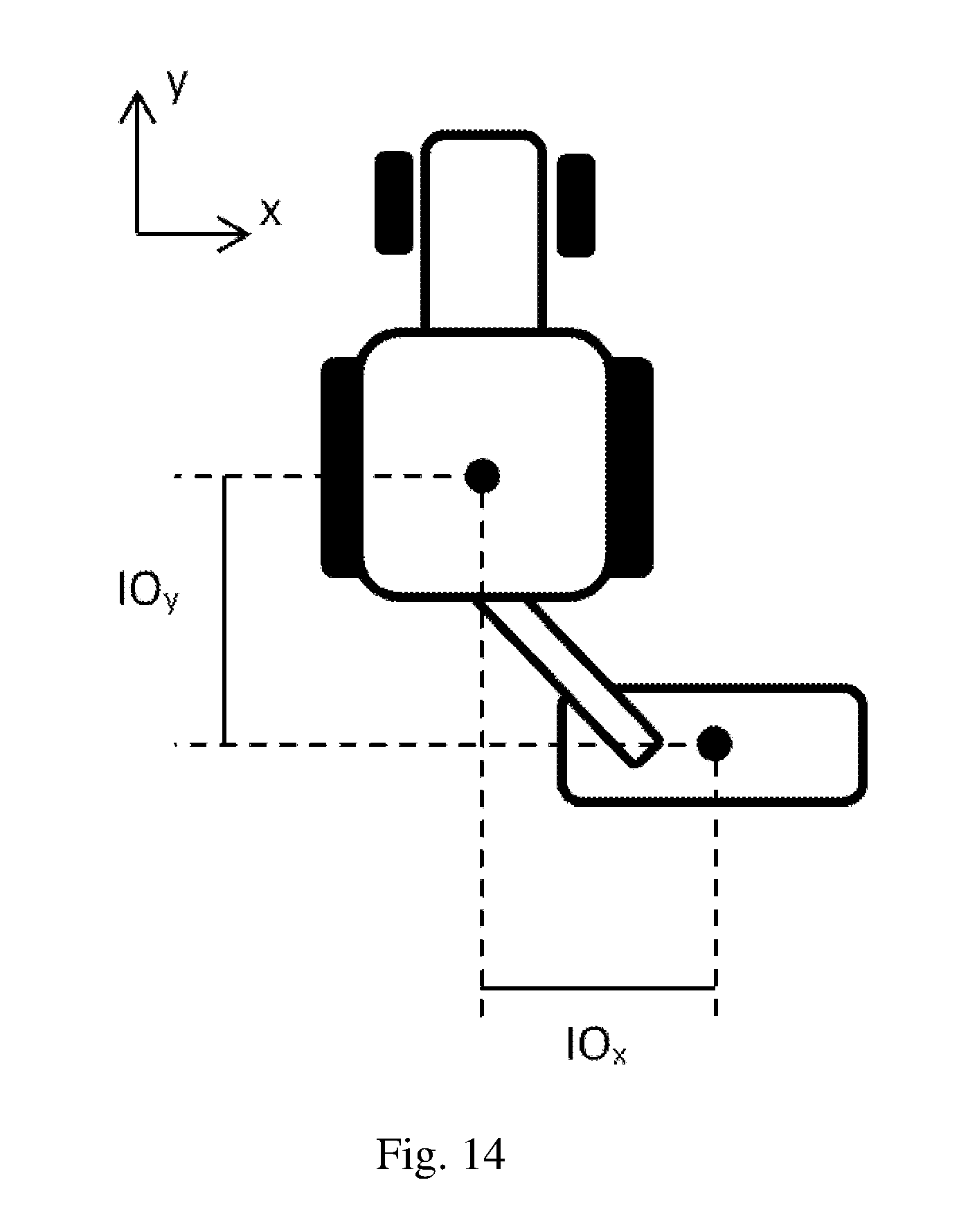
D00014

D00015
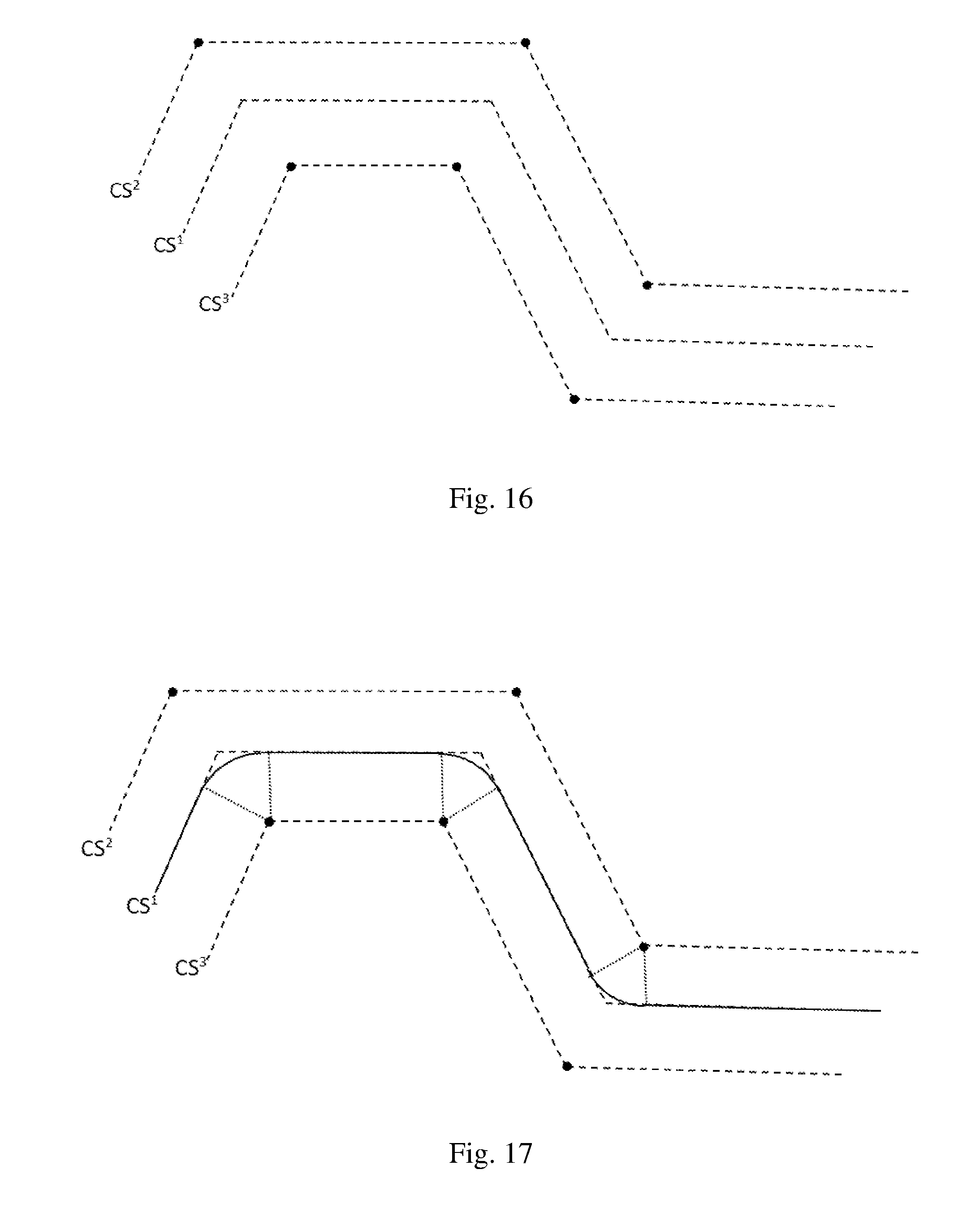
D00016
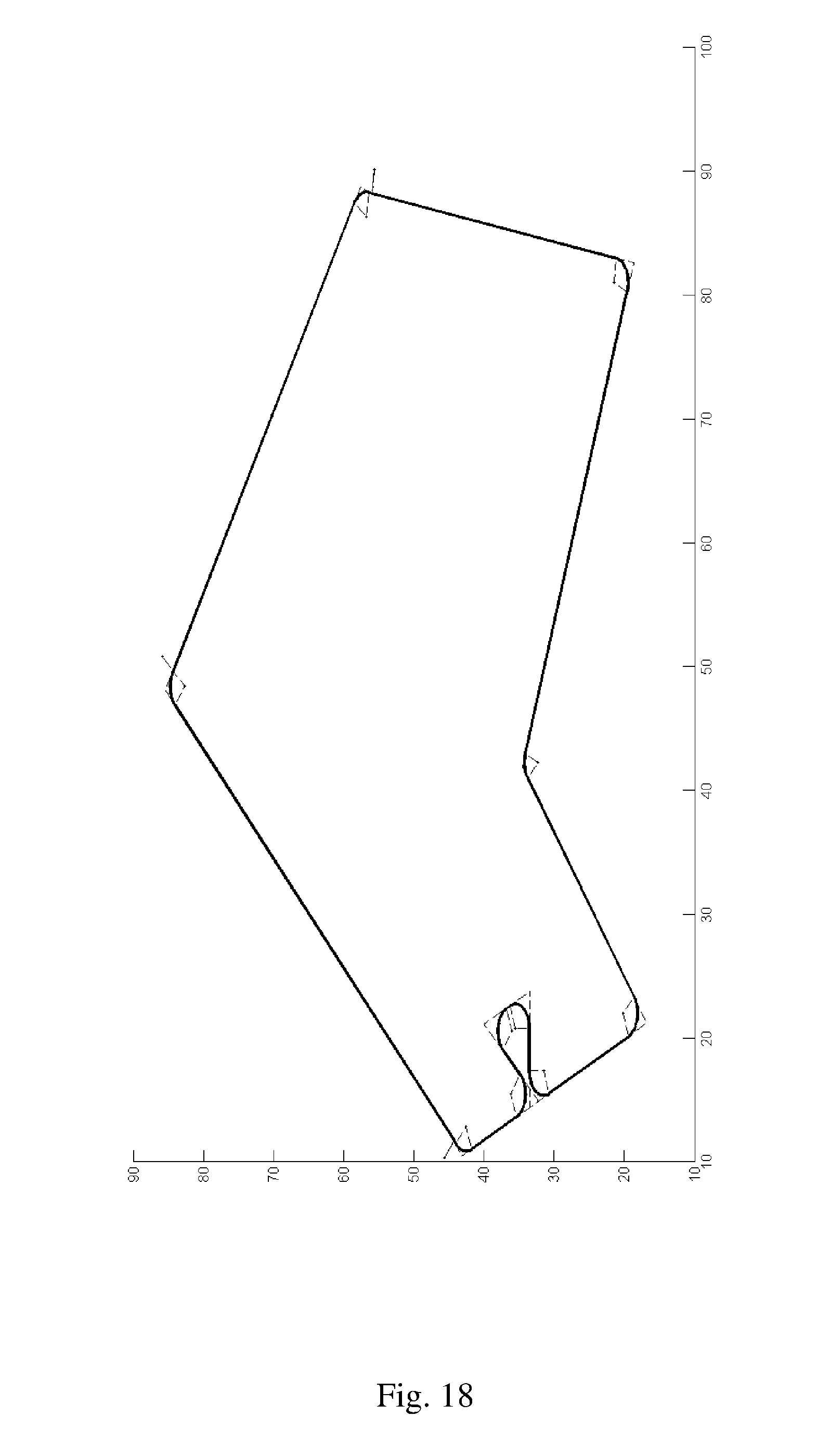
D00017

D00018
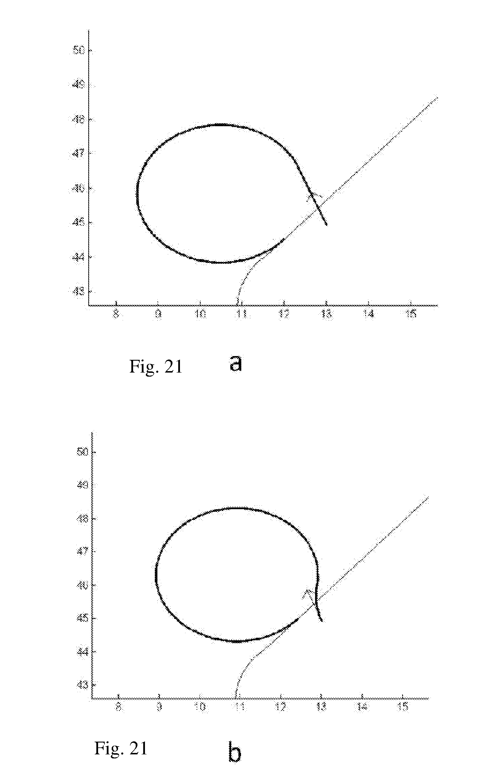
D00019
D00020

D00021
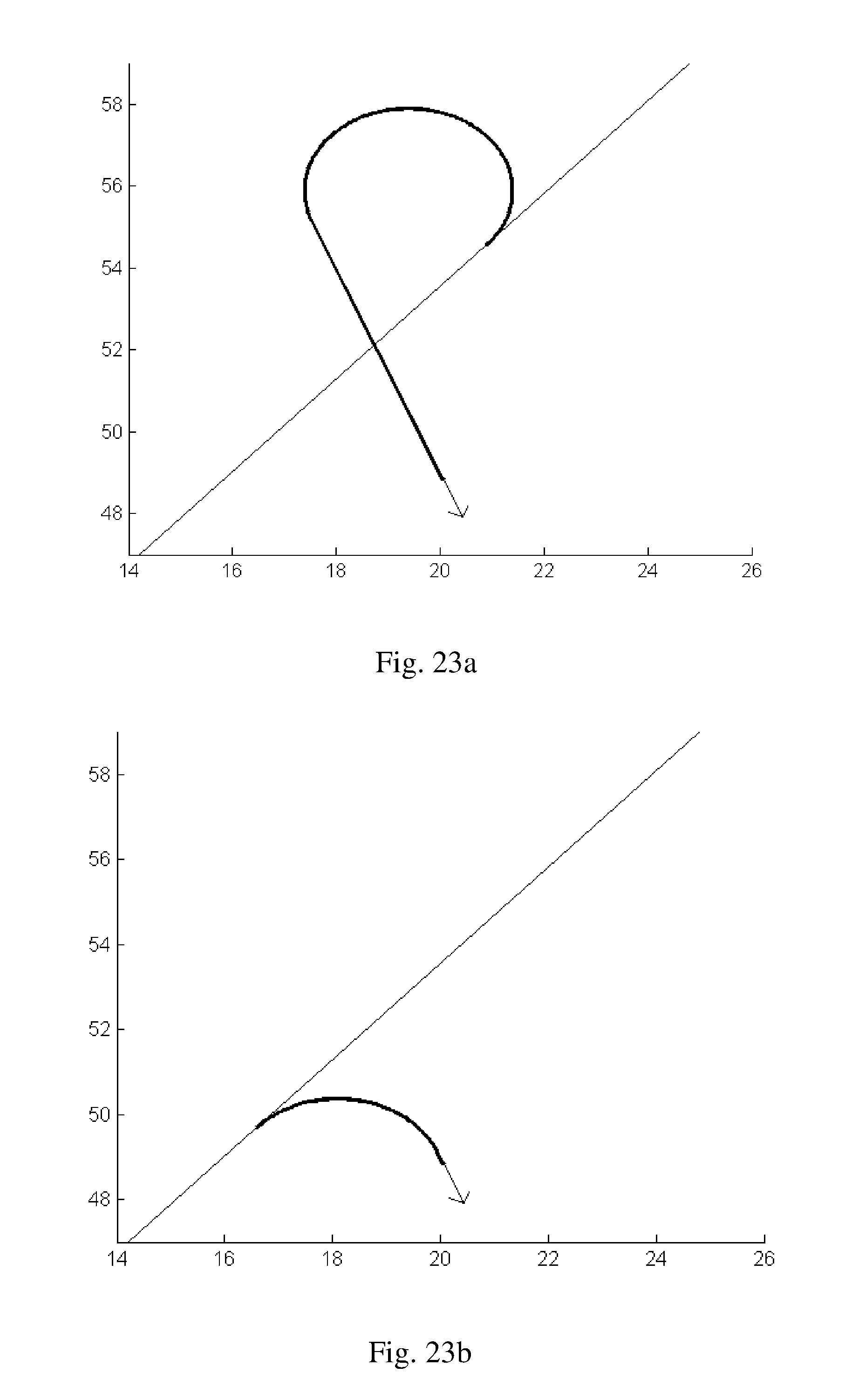
D00022

D00023

D00024
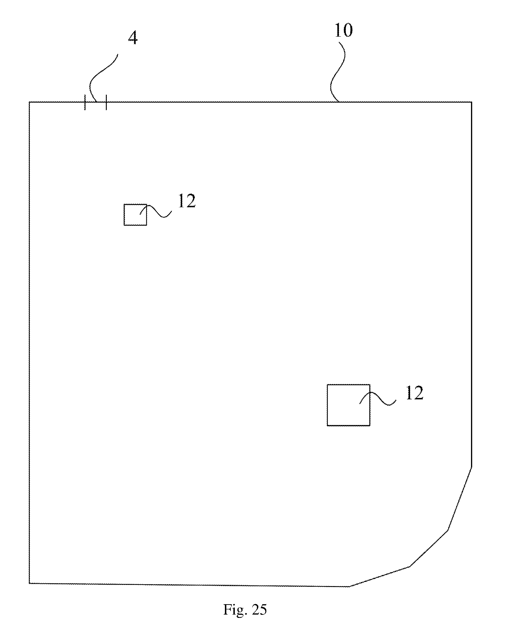
D00025
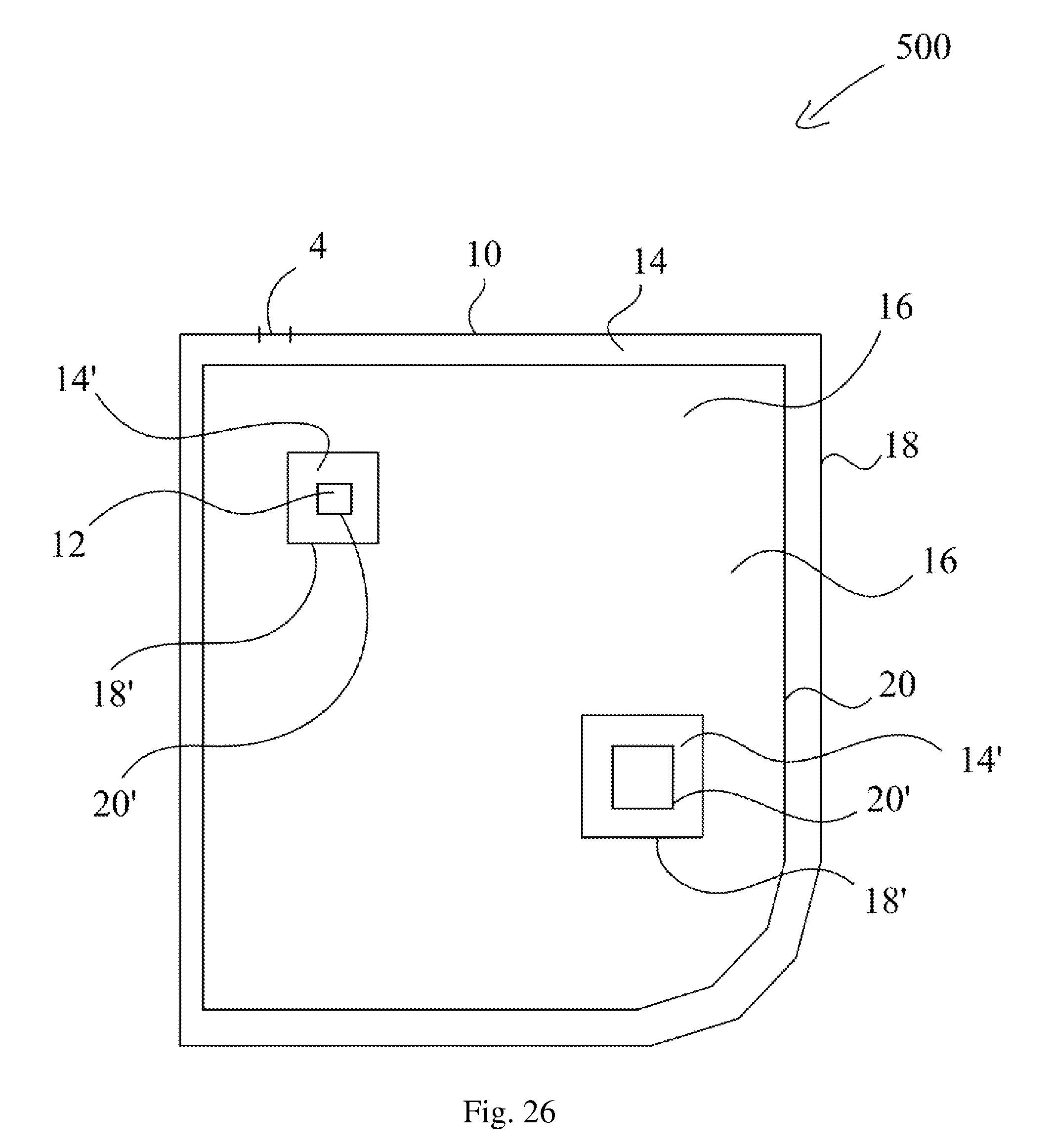
D00026
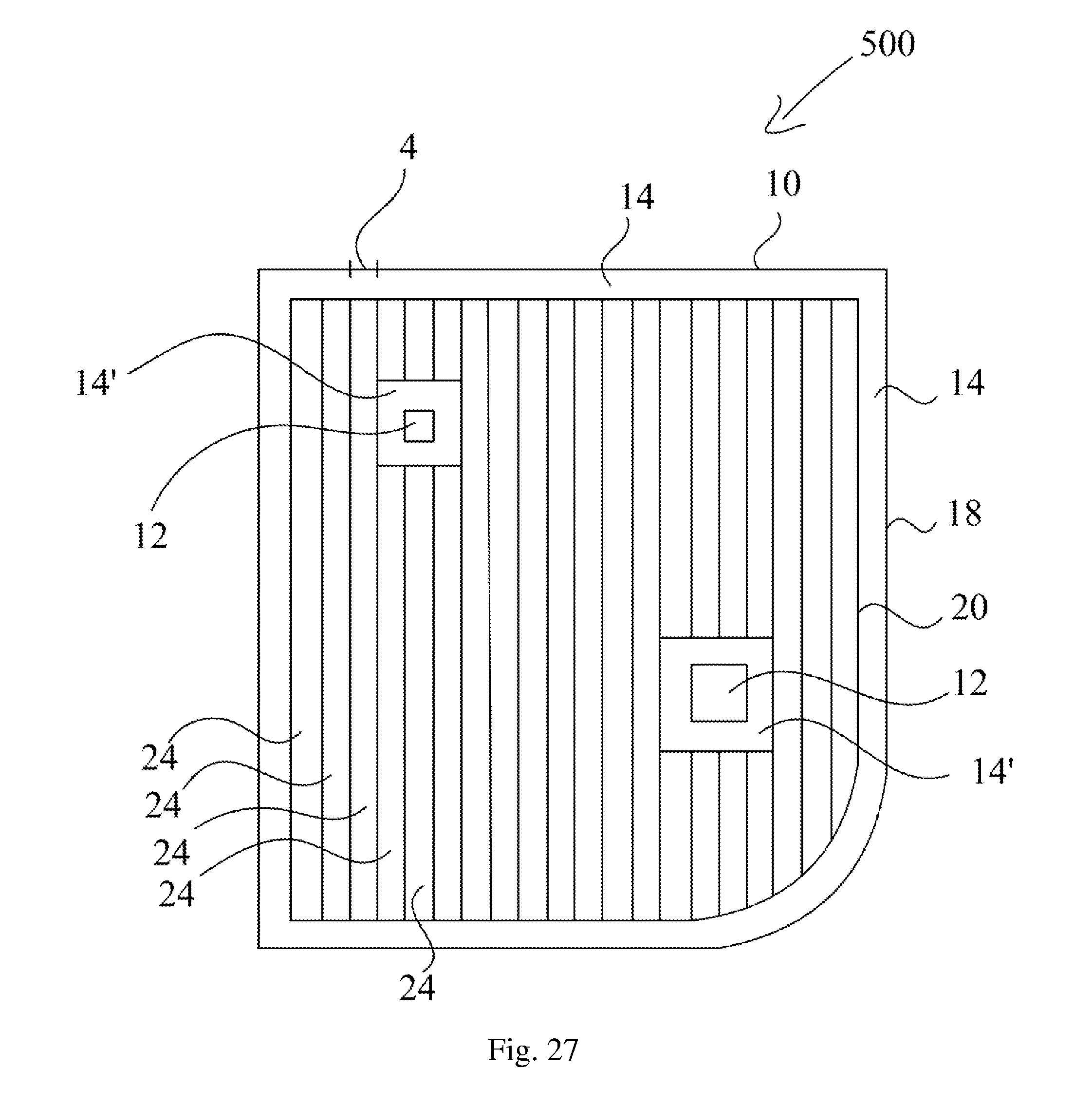
D00027

D00028

D00029
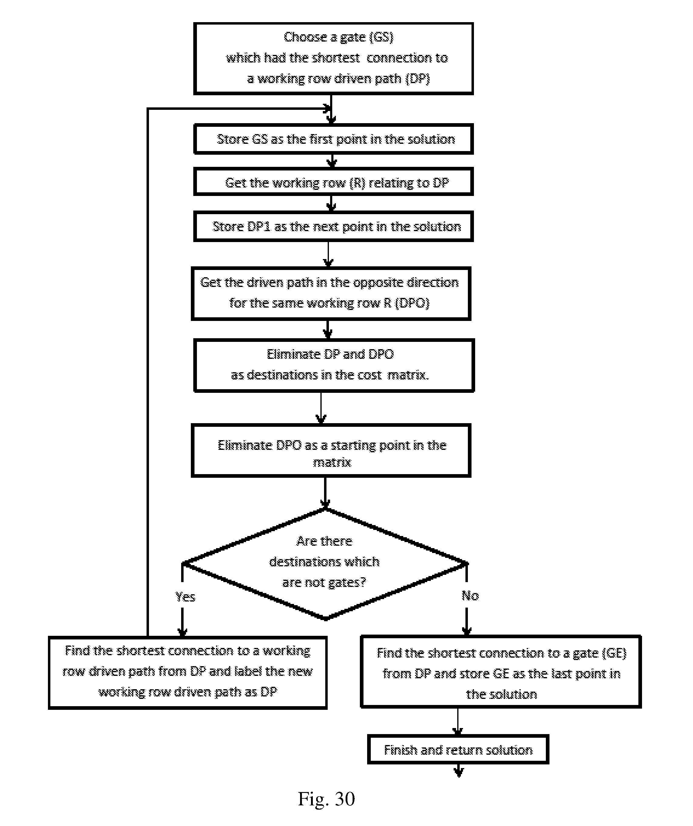


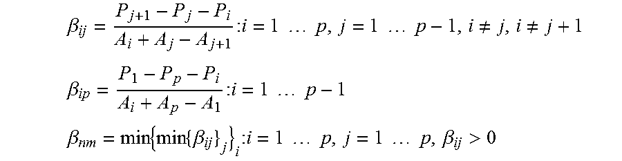
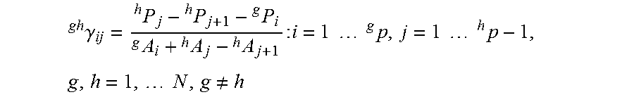

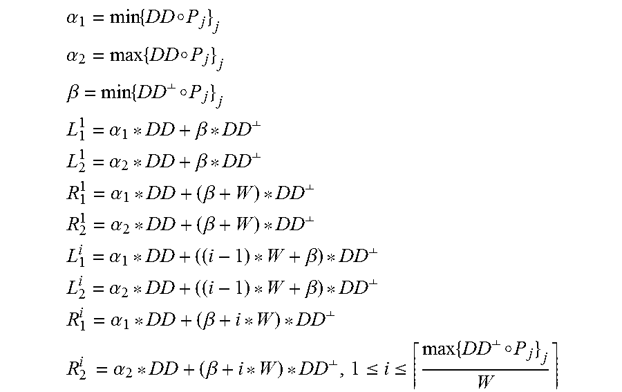

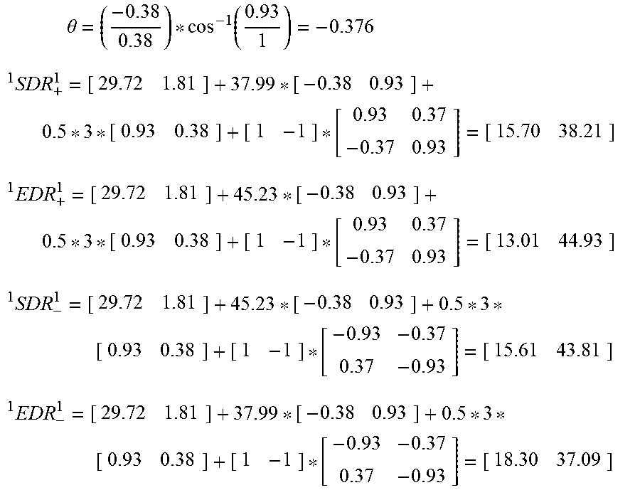

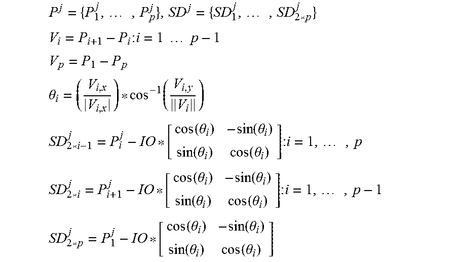

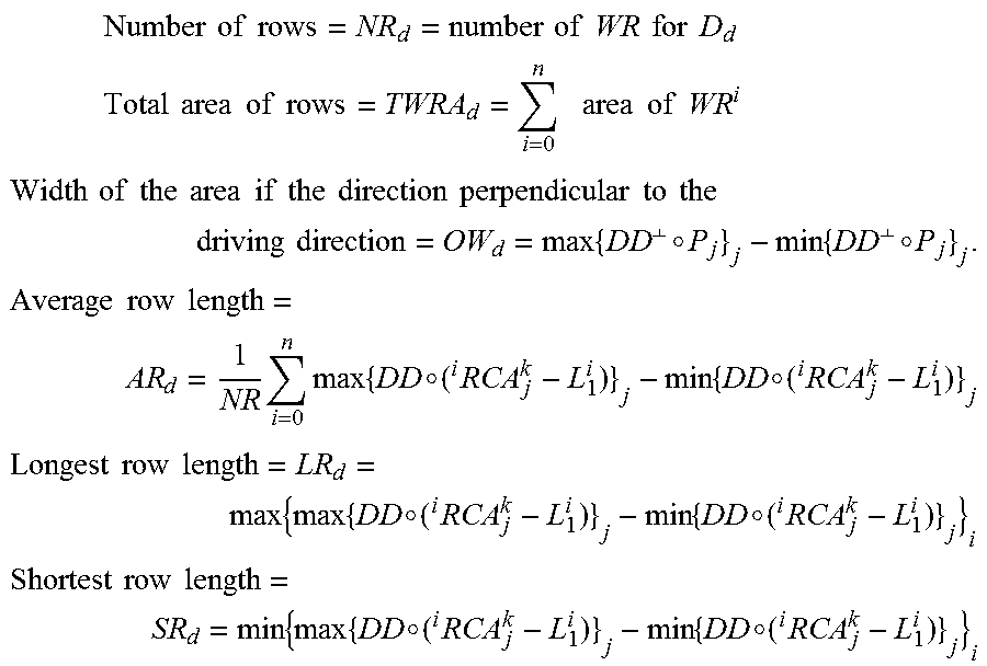
XML
uspto.report is an independent third-party trademark research tool that is not affiliated, endorsed, or sponsored by the United States Patent and Trademark Office (USPTO) or any other governmental organization. The information provided by uspto.report is based on publicly available data at the time of writing and is intended for informational purposes only.
While we strive to provide accurate and up-to-date information, we do not guarantee the accuracy, completeness, reliability, or suitability of the information displayed on this site. The use of this site is at your own risk. Any reliance you place on such information is therefore strictly at your own risk.
All official trademark data, including owner information, should be verified by visiting the official USPTO website at www.uspto.gov. This site is not intended to replace professional legal advice and should not be used as a substitute for consulting with a legal professional who is knowledgeable about trademark law.