System And Method For Combining Otfs With Qlo To Minimize Time-bandwidth Product
ASHRAFI; SOLYMAN
U.S. patent application number 16/216172 was filed with the patent office on 2019-06-13 for system and method for combining otfs with qlo to minimize time-bandwidth product. The applicant listed for this patent is NXGEN PARTNERS IP, LLC. Invention is credited to SOLYMAN ASHRAFI.
| Application Number | 20190182083 16/216172 |
| Document ID | / |
| Family ID | 66697452 |
| Filed Date | 2019-06-13 |


View All Diagrams
| United States Patent Application | 20190182083 |
| Kind Code | A1 |
| ASHRAFI; SOLYMAN | June 13, 2019 |
SYSTEM AND METHOD FOR COMBINING OTFS WITH QLO TO MINIMIZE TIME-BANDWIDTH PRODUCT
Abstract
A system for wirelessly transmitting data provides an input for receiving an input data stream. First modulation circuitry applies quantum level overlay (QLO) modulation to the input data stream to generate a QLO modulated data stream. Second modulation circuitry applies quantum level orthogonal time frequency space (OTFS) modulation to the QLO modulated data stream to create an OTFS/QLO modulated data stream. A transmitter transmits the OTFS/QLO modulated data stream.
| Inventors: | ASHRAFI; SOLYMAN; (PLANO, TX) | ||||||||||
| Applicant: |
|
||||||||||
|---|---|---|---|---|---|---|---|---|---|---|---|
| Family ID: | 66697452 | ||||||||||
| Appl. No.: | 16/216172 | ||||||||||
| Filed: | December 11, 2018 |
Related U.S. Patent Documents
| Application Number | Filing Date | Patent Number | ||
|---|---|---|---|---|
| 62598287 | Dec 13, 2017 | |||
| Current U.S. Class: | 1/1 |
| Current CPC Class: | H04L 25/03834 20130101; H04L 27/3488 20130101; H04L 25/03343 20130101; H04L 2025/03426 20130101; H04L 27/362 20130101; H04L 5/04 20130101 |
| International Class: | H04L 25/03 20060101 H04L025/03; H04L 27/36 20060101 H04L027/36 |
Claims
1. A system for wirelessly transmitting data, comprising: an input for receiving an input data stream; first modulation circuitry for applying quantum level overlay (QLO) modulation to the input data stream to generate a QLO modulated data stream; second modulation circuitry for applying quantum level orthogonal time frequency space (OTFS) modulation to the QLO modulated data stream to create an OTFS/QLO modulated data stream; and a transmitter for transmitting the OTFS/QLO modulated data stream.
2. The system of claim 1, further comprising: a receiver for receiving the OTFS/QLO modulated data stream; first demodulation circuitry for removing OTFS modulation from the OTFS/QLO modulated data stream to create the QLO modulated data stream; and second demodulation circuitry for removing QLO modulation from the QLO modulated data stream to create the input data stream.
3. The system of claim 2, wherein the first demodulation circuitry further implements the OFTS transform function and Wigner transform function.
4. The system of claim 1, wherein the QLO modulation minimizes the time-bandwidth product of the OTFS/QLO modulated data stream.
5. The system of claim 1, wherein the QLO modulation reduces Doppler shift and delay spread in the OTFS/QLO modulated data stream.
6. The system of claim 1, wherein the first modulation circuitry pegs a physical bandwidth to an order of the QLO function.
7. The system of claim 1, wherein the second modulation circuitry applies the QLO modulated signal to a bi-orthogonality condition.
8. The system of claim 7, wherein the bi-orthogonality condition is defined by the equation: .intg.g.sub.tx*(t)g.sub.rx(t-nT)e.sup.j2.pi.m.DELTA.f(t-nT)dt=.delta.(m).- delta.; and further wherein the QLO modulated data steam is used for the g.sub.rx and g.sub.rx functions.
9. The system of claim 1, wherein the second modulation circuitry further implements an OFTS transform function and a Heisenberg transform function.
10. The system of claim 8, wherein the OFTS transform function comprises mapping the QLO modulated data stream into a time-frequency domain and applying a symplectic finite Fourier transform (SFFT) to the mapped QLO modulated data stream.
11. A method for wirelessly transmitting data between a transmitter and a receiver, comprising: receiving at an input of the transmitter an input data stream; applying quantum level overlay (QLO) modulation to the input data stream to generate a QLO modulated data stream using first modulation circuitry; applying quantum level orthogonal time frequency space (OTFS) modulation to the QLO modulated data stream to create an OTFS/QLO modulated data stream using second modulation circuitry; and transmitting the OTFS/QLO modulated data stream from the transmitter.
12. The method of claim 11, further comprising: receiving the OTFS/QLO modulated data stream at the receiver; removing OTFS modulation from the OTFS/QLO modulated data stream to create the QLO modulated data stream using first demodulation circuitry; and removing QLO modulation from the QLO modulated data stream to create the input data stream using second demodulation circuitry.
13. The method of claim 12 further comprising the step of applying a Wigner transform to the OTFS/QLO modulated data stream after reception at the receiver.
14. The method of claim 11, wherein the QLO modulation minimizes the time-bandwidth product of the OTFS/QLO modulated data stream.
15. The method of claim 11, wherein the QLO modulation reduces Doppler shift and delay spread in the OTFS/QLO modulated data stream.
16. The method of claim 11, wherein the step of applying quantum level overlay (QLO) modulation further comprises pegging a physical bandwidth to an order of the QLO function.
17. The method of claim 11, wherein the step of applying the quantum level orthogonal time frequency space (OTFS) modulation further comprises applying the QLO modulated signal to a bi-orthogonality condition.
18. The method of claim 17, wherein the bi-orthogonality condition is defined by the equation: .intg.g.sub.tx*(t)g.sub.rx(t-nT)e.sup.j2.pi.m.DELTA.f(t-nT)dt=.delta.(m).- delta.; and further wherein the QLO modulated data steam is used for the g.sub.rx and g.sub.rx functions.
19. The method of claim 11, wherein the step of applying quantum level orthogonal time frequency space (OTFS) modulation further comprises: mapping the QLO modulated data stream into a time-frequency domain; and applying a symplectic finite Fourier transform (SFFT) to the mapped QLO modulated data stream.
20. The method of claim 11 further comprising the step of applying a Heisenberg transform to the OTFS/QLO modulated data stream prior to transmission.
21. A method for wirelessly transmitting data between a transmitter and a receiver, comprising: receiving at an input of the transmitter an input data stream; modulating the input data stream using Hermite-Gaussian signals to generate a first modulated data stream using first modulation circuitry; applying quantum level orthogonal time frequency space (OTFS) modulation to the first modulated data stream to create a second modulated data stream using second modulation circuitry; and transmitting the second modulated data stream from the transmitter.
22. The method of claim 21, further comprising: receiving the second modulated data stream at the receiver; removing OTFS modulation from the second modulated data stream to create the first modulated data stream using first demodulation circuitry; and removing modulation using the Hermite-Gaussian signals from the first modulated data stream to create the input data stream using second demodulation circuitry.
23. The method of claim 22 further comprising the step of applying a Wigner transform to the second modulated data stream after reception at the receiver.
24. The method of claim 21, wherein the modulation using the Hermite-Gaussian signals minimizes the time-bandwidth product of the second modulated data stream.
25. The method of claim 21, wherein the modulation using the Hermite-Gaussian signals reduces Doppler shift and delay spread in the OTFS/QLO modulated data stream.
26. The method of claim 21, wherein the step of modulating further comprises pegging a physical bandwidth to an order of the Hermite-Gaussian signals.
27. The method of claim 21, wherein the step of applying the quantum level orthogonal time frequency space (OTFS) modulation further comprises applying the first modulated signal to a bi-orthogonality condition.
28. The method of claim 27, wherein the bi-orthogonality condition is defined by the equation: .intg.g.sub.tx*(t)g.sub.rx(t-nT)e.sup.j2.pi.m.DELTA.f(t-nT)dt=.delta.(m).- delta.; and further wherein the first modulated data steam is used for the g.sub.rx and g.sub.rx functions.
29. The method of claim 21, wherein the step of applying quantum level orthogonal time frequency space (OTFS) modulation further comprises: mapping the first modulated data stream into a time-frequency domain; and applying a symplectic finite Fourier transform (SFFT) to the mapped first modulated data stream.
30. The method of claim 21 further comprising the step of applying a Heisenberg transform to the second modulated data stream prior to transmission.
Description
CROSS-REFERENCE TO RELATED APPLICATIONS
[0001] This application claims priority to U.S. Provisional Application No. 62/598,287, entitled SYSTEM AND METHOD FOR COMBINING OTFS WITH QLO TO MINIMIZE TIME-BANDWIDTH PRODUCT (Atty. Dkt. No. NXGN60-33951), filed on Dec. 12, 2017, which is incorporated by reference herein in its entirety.
TECHNICAL FIELD
[0002] The following disclosure relates to systems and methods for reducing dispersive frequency channels caused by Doppler spread, and more particularly to reducing dispersive frequency channels caused by Doppler spread using a combination of multiple layer overlay modulation and orthogonal time frequency space modulation.
BACKGROUND
[0003] The use of voice and data networks has greatly increased as the number of personal computing and communication devices, such as laptop computers, mobile telephones, Smartphones, tablets, et cetera, has grown. The astronomically increasing number of personal mobile communication devices has concurrently increased the amount of data being transmitted over the networks providing infrastructure for these mobile communication devices. As these mobile communication devices become more ubiquitous in business and personal lifestyles, the abilities of these networks to support all of the new users and user devices has been strained. Thus, a major concern of network infrastructure providers is the ability to increase their bandwidth and limit interference in order to support the greater load of voice and data communications and particularly videos that are occurring. Traditional manners for increasing the bandwidth in such systems have involved increasing the number of channels so that a greater number of communications may be transmitted, or increasing the speed at which information is transmitted over existing channels in order to provide greater throughput levels over the existing channel resources.
SUMMARY
[0004] The present invention, as disclosed and describe herein, in one aspect thereof, comprises a system for wirelessly transmitting data provides an input for receiving an input data stream. First modulation circuitry applies quantum level overlay (QLO) modulation to the input data stream to generate a QLO modulated data stream. Second modulation circuitry applies quantum level orthogonal time frequency space (OTFS) modulation to the QLO modulated data stream to create an OTFS/QLO modulated data stream. A transmitter transmits the OTFS/QLO modulated data stream.
BRIEF DESCRIPTION OF THE DRAWINGS
[0005] For a more complete understanding, reference is now made to the following description taken in conjunction with the accompanying Drawings in which:
[0006] FIG. 1 illustrates various techniques for increasing spectral efficiency within a transmitted signal;
[0007] FIG. 2 illustrates a particular technique for increasing spectral efficiency within a transmitted signal;
[0008] FIG. 3 illustrates a general overview of the manner for providing communication bandwidth between various communication protocol interfaces;
[0009] FIG. 4 illustrates the manner for utilizing multiple level overlay modulation with twisted pair/cable interfaces;
[0010] FIG. 5 illustrates a general block diagram for processing a plurality of data streams within an optical communication system;
[0011] FIG. 6 is a functional block diagram of a system for generating orbital angular momentum within a communication system;
[0012] FIG. 7 is a functional block diagram of the orbital angular momentum signal processing block of FIG. 6;
[0013] FIG. 8 is a functional block diagram illustrating the manner for removing orbital angular momentum from a received signal including a plurality of data streams;
[0014] FIG. 9 illustrates a single wavelength having two quanti-spin polarizations providing an infinite number of signals having various orbital angular momentums associated therewith;
[0015] FIG. 10A illustrates a plane wave having only variations in the spin angular momentum;
[0016] FIG. 10B illustrates a signal having both spin and orbital angular momentum applied thereto;
[0017] FIGS. 11A-11C illustrate various signals having different orbital angular momentum applied thereto;
[0018] FIG. 11D illustrates a propagation of Poynting vectors for various Eigen modes;
[0019] FIG. 11E illustrates a spiral phase plate;
[0020] FIG. 12 illustrates a multiple level overlay modulation system;
[0021] FIG. 13 illustrates a multiple level overlay demodulator;
[0022] FIG. 14 illustrates a multiple level overlay transmitter system;
[0023] FIG. 15 illustrates a multiple level overlay receiver system;
[0024] FIGS. 16A-16K illustrate representative multiple level overlay signals and their respective spectral power densities;
[0025] FIG. 17 illustrates comparisons of multiple level overlay signals within the time and frequency domain;
[0026] FIG. 18 illustrates a spectral alignment of multiple level overlay signals for differing bandwidths of signals;
[0027] FIG. 19 illustrates an alternative spectral alignment of multiple level overlay signals;
[0028] FIG. 20 illustrates power spectral density for various signal layers using a combined three layer multiple level overlay technique;
[0029] FIG. 21 illustrates power spectral density on a log scale for layers using a combined three layer multiple level overlay modulation;
[0030] FIG. 22 illustrates a bandwidth efficiency comparison for square root raised cosine versus multiple layer overlay for a symbol rate of 1/6;
[0031] FIG. 23 illustrates a bandwidth efficiency comparison between square root raised cosine and multiple layer overlay for a symbol rate of 1/4;
[0032] FIG. 24 illustrates a performance comparison between square root raised cosine and multiple level overlay using ACLR;
[0033] FIG. 25 illustrates a performance comparison between square root raised cosine and multiple lever overlay using out of band power;
[0034] FIG. 26 illustrates a performance comparison between square root raised cosine and multiple lever overlay using band edge PSD;
[0035] FIG. 27 is a block diagram of a transmitter subsystem for use with multiple level overlay;
[0036] FIG. 28 is a block diagram of a receiver subsystem using multiple level overlay;
[0037] FIG. 29 illustrates an equivalent discreet time orthogonal channel of modified multiple level overlay;
[0038] FIG. 30 illustrates the PSDs of multiple layer overlay, modified multiple layer overlay and square root raised cosine;
[0039] FIG. 31 illustrates a bandwidth comparison based on -40 dBc out of band power bandwidth between multiple layer overlay and square root raised cosine;
[0040] FIG. 32 illustrates equivalent discrete time parallel orthogonal channels of modified multiple layer overlay;
[0041] FIG. 33 illustrates the channel power gain of the parallel orthogonal channels of modified multiple layer overlay with three layers and T.sub.sym=3;
[0042] FIG. 34 illustrates a spectral efficiency comparison based on ACLR1 between modified multiple layer overlay and square root raised cosine;
[0043] FIG. 35 illustrates a spectral efficiency comparison between modified multiple layer overlay and square root raised cosine based on OBP;
[0044] FIG. 36 illustrates a spectral efficiency comparison based on ACLR1 between modified multiple layer overlay and square root raised cosine;
[0045] FIG. 37 illustrates a spectral efficiency comparison based on OBP between modified multiple layer overlay and square root raised cosine;
[0046] FIG. 38 illustrates a block diagram of a baseband transmitter for a low pass equivalent modified multiple layer overlay system;
[0047] FIG. 39 illustrates a block diagram of a baseband receiver for a low pass equivalent modified multiple layer overlay system;
[0048] FIG. 40 illustrates a block diagram of a combination of quantum level overlay (QLO) and orthogonal time frequency space (OTFS) modulations;
[0049] FIG. 41 illustrates a block diagram of OTFS modulation; and
[0050] FIG. 42 illustrates a block diagram of QLO and OTFS modulations.
DETAILED DESCRIPTION
[0051] Referring now to the drawings, wherein like reference numbers are used herein to designate like elements throughout, the various views and embodiments of system and method for communication using orbital angular momentum with modulation are illustrated and described, and other possible embodiments are described. The figures are not necessarily drawn to scale, and in some instances the drawings have been exaggerated and/or simplified in places for illustrative purposes only. One of ordinary skill in the art will appreciate the many possible applications and variations based on the following examples of possible embodiments.
[0052] Referring now to the drawings, and more particularly to FIG. 1, wherein there is illustrated two manners for increasing spectral efficiency of a communications system. In general, there are basically two ways to increase spectral efficiency 102 of a communications system. The increase may be brought about by signal processing techniques 104 in the modulation scheme or using multiple access technique. Additionally, the spectral efficiency can be increase by creating new Eigen channels 106 within the electromagnetic propagation. These two techniques are completely independent of one another and innovations from one class can be added to innovations from the second class. Therefore, the combination of this technique introduced a further innovation.
[0053] Spectral efficiency 102 is the key driver of the business model of a communications system. The spectral efficiency is defined in units of bit/sec/hz and the higher the spectral efficiency, the better the business model. This is because spectral efficiency can translate to a greater number of users, higher throughput, higher quality or some of each within a communications system.
[0054] Regarding techniques using signal processing techniques or multiple access techniques. These techniques include innovations such as TDMA, FDMA, CDMA, EVDO, GSM, WCDMA, HSPA and the most recent OFDM techniques used in 4G WIMAX and LTE. Almost all of these techniques use decades-old modulation techniques based on sinusoidal Eigen functions called QAM modulation. Within the second class of techniques involving the creation of new Eigen channels 106, the innovations include diversity techniques including space and polarization diversity as well as multiple input/multiple output (MIMO) where uncorrelated radio paths create independent Eigen channels and propagation of electromagnetic waves.
[0055] Referring now to FIG. 2, the present communication system configuration introduces two techniques, one from the signal processing techniques 104 category and one from the creation of new eigen channels 106 category that are entirely independent from each other. Their combination provides a unique manner to disrupt the access part of an end to end communications system from twisted pair and coaxial cable to fiber optics, to free space optics, to RF used in cellular, backhaul and satellite including but not limited to Point-to-Point, Point-to-Multipoint, Point-to-Point (Backhaul), Point-to-Point (Fronthaul--higher throughput CPRI interface for cloudification and virtualization of RAN and future cloudified HetNet), broadcast, internet of things (TOT), Wifi (LAN), Bluetooth (PAN), personal devices cable replacement, RF and FSO hybrid system and radar. The first technique involves the use of a new signal processing technique using new orthogonal signals to upgrade QAM modulation using non sinusoidal functions. This is referred to as quantum level overlay (QLO) 202. The second technique involves the application of new electromagnetic wavefronts using a property of electromagnetic waves or photon, called orbital angular momentum (QAM) 104. Application of each of the quantum level overlay techniques 202 and orbital angular momentum application 204 uniquely offers orders of magnitude higher spectral efficiency 206 within communication systems in their combination.
[0056] With respect to the quantum level overlay technique 202, new eigen functions are introduced that when overlapped (on top of one another within a symbol) significantly increases the spectral efficiency of the system. The quantum level overlay technique 302 borrows from quantum mechanics, special orthogonal signals that reduce the time bandwidth product and thereby increase the spectral efficiency of the channel. Each orthogonal signal is overlaid within the symbol acts as an independent channel. These independent channels differentiate the technique from existing modulation techniques.
[0057] With respect to the application of orbital angular momentum 204, this technique introduces twisted electromagnetic waves, or light beams, having helical wave fronts that carry orbital angular momentum (OAM). Different OAM carrying waves/beams can be mutually orthogonal to each other within the spatial domain, allowing the waves/beams to be efficiently multiplexed and demultiplexed within a communications link. OAM beams are interesting in communications due to their potential ability in special multiplexing multiple independent data carrying channels.
[0058] With respect to the combination of quantum level overlay techniques 202 and orbital angular momentum application 204, the combination is unique as the OAM multiplexing technique is compatible with other electromagnetic techniques such as wave length and polarization division multiplexing. This suggests the possibility of further increasing system performance. The application of these techniques together in high capacity data transmission disrupts the access part of an end to end communications system from twisted pair and cable to fiber optics, to free space optics, to RF used in cellular/backhaul and satellites.
[0059] Each of these techniques can be applied independent of one another, but the combination provides a unique opportunity to not only increase spectral efficiency, but to increase spectral efficiency without sacrificing distance or signal to noise ratios.
[0060] Using the Shannon Capacity Equation, a determination may be made if spectral efficiency is increased. This can be mathematically translated to more bandwidth. Since bandwidth has a value, one can easily convert spectral efficiency gains to financial gains for the business impact of using higher spectral efficiency. Also, when sophisticated forward error correction (FEC) techniques are used, the net impact is higher quality but with the sacrifice of some bandwidth. However, if one can achieve higher spectral efficiency (or more virtual bandwidth), one can sacrifice some of the gained bandwidth for FEC and therefore higher spectral efficiency can also translate to higher quality.
[0061] Telecom operators and vendors are interested in increasing spectral efficiency. However, the issue with respect to this increase is the cost. Each technique at different layers of the protocol has a different price tag associated therewith. Techniques that are implemented at a physical layer have the most impact as other techniques can be superimposed on top of the lower layer techniques and thus increase the spectral efficiency further. The price tag for some of the techniques can be drastic when one considers other associated costs. For example, the multiple input multiple output (MIMO) technique uses additional antennas to create additional paths where each RF path can be treated as an independent channel and thus increase the aggregate spectral efficiency. In the MIMO scenario, the operator has other associated soft costs dealing with structural issues such as antenna installations, etc. These techniques not only have tremendous cost, but they have huge timing issues as the structural activities take time and the achieving of higher spectral efficiency comes with significant delays which can also be translated to financial losses.
[0062] The quantum level overlay technique 202 has an advantage that the independent channels are created within the symbols without needing new antennas. This will have a tremendous cost and time benefit compared to other techniques. Also, the quantum layer overlay technique 202 is a physical layer technique, which means there are other techniques at higher layers of the protocol that can all ride on top of the QLO techniques 202 and thus increase the spectral efficiency even further. QLO technique 202 uses standard QAM modulation used in OFDM based multiple access technologies such as WIMAX or LTE. QLO technique 202 basically enhances the QAM modulation at the transceiver by injecting new signals to the I & Q components of the baseband and overlaying them before QAM modulation as will be more fully described herein below. At the receiver, the reverse procedure is used to separate the overlaid signal and the net effect is a pulse shaping that allows better localization of the spectrum compared to standard QAM or even the root raised cosine. The impact of this technique is a significantly higher spectral efficiency.
[0063] Referring now more particularly to FIG. 3, there is illustrated a general overview of the manner for providing improved communication bandwidth within various communication protocol interfaces 302, using a combination of multiple level overlay modulation 304 and the application of orbital angular momentum 306 to increase the number of communications channels.
[0064] The various communication protocol interfaces 302 may comprise a variety of communication links, such as RF communication, wireline communication such as cable or twisted pair connections, or optical communications making use of light wavelengths such as fiber-optic communications or free-space optics. Various types of RF communications may include a combination of RF microwave or RF satellite communication, as well as multiplexing between RF and free-space optics in real time.
[0065] By combining a multiple layer overlay modulation technique 304 with orbital angular momentum (OAM) technique 306, a higher throughput over various types of communication links 302 may be achieved. The use of multiple level overlay modulation alone without OAM increases the spectral efficiency of communication links 302, whether wired, optical, or wireless. However, with OAM, the increase in spectral efficiency is even more significant.
[0066] Multiple overlay modulation techniques 304 provide a new degree of freedom beyond the conventional 2 degrees of freedom, with time T and frequency F being independent variables in a two-dimensional notational space defining orthogonal axes in an information diagram. This comprises a more general approach rather than modeling signals as fixed in either the frequency or time domain. Previous modeling methods using fixed time or fixed frequency are considered to be more limiting cases of the general approach of using multiple level overlay modulation 304. Within the multiple level overlay modulation technique 304, signals may be differentiated in two-dimensional space rather than along a single axis. Thus, the information-carrying capacity of a communications channel may be determined by a number of signals which occupy different time and frequency coordinates and may be differentiated in a notational two-dimensional space.
[0067] Within the notational two-dimensional space, minimization of the time bandwidth product, i.e., the area occupied by a signal in that space, enables denser packing, and thus, the use of more signals, with higher resulting information-carrying capacity, within an allocated channel. Given the frequency channel delta (.DELTA.f), a given signal transmitted through it in minimum time .DELTA.t will have an envelope described by certain time-bandwidth minimizing signals. The time-bandwidth products for these signals take the form;
.DELTA.t.DELTA.f=1/2(2n+1)
where n is an integer ranging from 0 to infinity, denoting the order of the signal.
[0068] These signals form an orthogonal set of infinite elements, where each has a finite amount of energy. They are finite in both the time domain and the frequency domain, and can be detected from a mix of other signals and noise through correlation, for example, by match filtering. Unlike other wavelets, these orthogonal signals have similar time and frequency forms.
[0069] The orbital angular momentum process 306 provides a twist to wave fronts of the electromagnetic fields carrying the data stream that may enable the transmission of multiple data streams on the same frequency, wavelength, or other signal-supporting mechanism. This will increase the bandwidth over a communications link by allowing a single frequency or wavelength to support multiple eigen channels, each of the individual channels having a different orthogonal and independent orbital angular momentum associated therewith.
[0070] Referring now to FIG. 4, there is illustrated a further communication implementation technique using the above described techniques as twisted pairs or cables carry electrons (not photons). Rather than using each of the multiple level overlay modulation 304 and orbital angular momentum techniques 306, only the multiple level overlay modulation 304 can be used in conjunction with a single wireline interface and, more particularly, a twisted pair communication link or a cable communication link 402. The operation of the multiple level overlay modulation 404, is similar to that discussed previously with respect to FIG. 3, but is used by itself without the use of orbital angular momentum techniques 306, and is used with either a twisted pair communication link or cable interface communication link 402.
[0071] Referring now to FIG. 5, there is illustrated a general block diagram for processing a plurality of data streams 502 for transmission in an optical communication system. The multiple data streams 502 are provided to the multi-layer overlay modulation circuitry 504 wherein the signals are modulated using the multi-layer overlay modulation technique. The modulated signals are provided to orbital angular momentum processing circuitry 506 which applies a twist to each of the wave fronts being transmitted on the wavelengths of the optical communication channel. The twisted waves are transmitted through the optical interface 508 over an optical communications link such as an optical fiber or free space optics communication system. FIG. 5 may also illustrate an RF mechanism wherein the interface 508 would comprise and RF interface rather than an optical interface.
[0072] Referring now more particularly to FIG. 6, there is illustrated a functional block diagram of a system for generating the orbital angular momentum "twist" within a communication system, such as that illustrated with respect to FIG. 3, to provide a data stream that may be combined with multiple other data streams for transmission upon a same wavelength or frequency. Multiple data streams 602 are provided to the transmission processing circuitry 600. Each of the data streams 602 comprises, for example, an end to end link connection carrying a voice call or a packet connection transmitting non-circuit switch packed data over a data connection. The multiple data streams 602 are processed by modulator/demodulator circuitry 604. The modulator/demodulator circuitry 604 modulates the received data stream 602 onto a wavelength or frequency channel using a multiple level overlay modulation technique, as will be more fully described herein below. The communications link may comprise an optical fiber link, free-space optics link, RF microwave link, RF satellite link, wired link (without the twist), etc.
[0073] The modulated data stream is provided to the orbital angular momentum (OAM) signal processing block 606. Each of the modulated data streams from the modulator/demodulator 604 are provided a different orbital angular momentum by the orbital angular momentum electromagnetic block 606 such that each of the modulated data streams have a unique and different orbital angular momentum associated therewith. Each of the modulated signals having an associated orbital angular momentum are provided to an optical transmitter 608 that transmits each of the modulated data streams having a unique orbital angular momentum on a same wavelength. Each wavelength has a selected number of bandwidth slots B and may have its data transmission capability increase by a factor of the number of degrees of orbital angular momentum e that are provided from the OAM electromagnetic block 606. The optical transmitter 608 transmitting signals at a single wavelength could transmit B groups of information. The optical transmitter 608 and OAM electromagnetic block 606 may transmit l.times.B groups of information according to the configuration described herein.
[0074] In a receiving mode, the optical transmitter 608 will have a wavelength including multiple signals transmitted therein having different orbital angular momentum signals embedded therein. The optical transmitter 608 forwards these signals to the OAM signal processing block 606, which separates each of the signals having different orbital angular momentum and provides the separated signals to the demodulator circuitry 604. The demodulation process extracts the data streams 602 from the modulated signals and provides it at the receiving end using the multiple layer overlay demodulation technique.
[0075] Referring now to FIG. 7, there is provided a more detailed functional description of the OAM signal processing block 606. Each of the input data streams are provided to OAM circuitry 702. Each of the OAM circuitry 702 provides a different orbital angular momentum to the received data stream. The different orbital angular momentums are achieved by applying different currents for the generation of the signals that are being transmitted to create a particular orbital angular momentum associated therewith. The orbital angular momentum provided by each of the OAM circuitries 702 are unique to the data stream that is provided thereto. An infinite number of orbital angular momentums may be applied to different input data streams using many different currents. Each of the separately generated data streams are provided to a signal combiner 704, which combines the signals onto a wavelength for transmission from the transmitter 706.
[0076] Referring now to FIG. 8, there is illustrated the manner in which the OAM processing circuitry 606 may separate a received signal into multiple data streams. The receiver 802 receives the combined OAM signals on a single wavelength and provides this information to a signal separator 804. The signal separator 804 separates each of the signals having different orbital angular momentums from the received wavelength and provides the separated signals to OAM de-twisting circuitry 806. The OAM de-twisting circuitry 806 removes the associated OAM twist from each of the associated signals and provides the received modulated data stream for further processing. The signal separator 804 separates each of the received signals that have had the orbital angular momentum removed therefrom into individual received signals. The individually received signals are provided to the receiver 802 for demodulation using, for example, multiple level overlay demodulation as will be more fully described herein below.
[0077] FIG. 9 illustrates in a manner in which a single wavelength or frequency, having two quanti-spin polarizations may provide an infinite number of twists having various orbital angular momentums associated therewith. The/axis represents the various quantized orbital angular momentum states which may be applied to a particular signal at a selected frequency or wavelength. The symbol omega (w) represents the various frequencies to which the signals of differing orbital angular momentum may be applied. The top grid 902 represents the potentially available signals for a left handed signal polarization, while the bottom grid 904 is for potentially available signals having right handed polarization.
[0078] By applying different orbital angular momentum states to a signal at a particular frequency or wavelength, a potentially infinite number of states may be provided at the frequency or wavelength. Thus, the state at the frequency .DELTA..omega. or wavelength 906 in both the left handed polarization plane 902 and the right handed polarization plane 904 can provide an infinite number of signals at different orbital angular momentum states .DELTA.l. Blocks 908 and 910 represent a particular signal having an orbital angular momentum .DELTA.l at a frequency .DELTA..omega. or wavelength in both the right handed polarization plane 904 and left handed polarization plane 910, respectively. By changing to a different orbital angular momentum within the same frequency .DELTA..omega. or wavelength 906, different signals may also be transmitted. Each angular momentum state corresponds to a different determined current level for transmission from the optical transmitter. By estimating the equivalent current for generating a particular orbital angular momentum within the optical domain and applying this current for transmission of the signals, the transmission of the signal may be achieved at a desired orbital angular momentum state.
[0079] Thus, the illustration of FIG. 9, illustrates two possible angular momentums, the spin angular momentum, and the orbital angular momentum. The spin version is manifested within the polarizations of macroscopic electromagnetism, and has only left and right hand polarizations due to up and down spin directions. However, the orbital angular momentum indicates an infinite number of states that are quantized. The paths are more than two and can theoretically be infinite through the quantized orbital angular momentum levels.
[0080] Using the orbital angular momentum state of the transmitted energy signals, physical information can be embedded within the radiation transmitted by the signals. The Maxwell-Heaviside equations can be represented as:
.gradient. E = .rho. 0 ##EQU00001## .gradient. .times. E - .differential. B .differential. t ##EQU00001.2## .gradient. B = 0 ##EQU00001.3## .gradient. .times. B = 0 .mu. 0 .differential. E .differential. t + .mu. 0 j ( t , x ) ##EQU00001.4##
where .gradient. is the del operator, E is the electric field intensity and B is the magnetic flux density. Using these equations, one can derive 23 symmetries/conserved quantities from Maxwell's original equations. However, there are only ten well-known conserved quantities and only a few of these are commercially used. Historically if Maxwell's equations where kept in their original quaternion forms, it would have been easier to see the symmetries/conserved quantities, but when they were modified to their present vectorial form by Heaviside, it became more difficult to see such inherent symmetries in Maxwell's equations.
[0081] Maxwell's linear theory is of U(1) symmetry with Abelian commutation relations. They can be extended to higher symmetry group SU(2) form with non-Abelian commutation relations that address global (non-local in space) properties. The Wu-Yang and Harmuth interpretation of Maxwell's theory implicates the existence of magnetic monopoles and magnetic charges. As far as the classical fields are concerned, these theoretical constructs are pseudo-particle, or instanton. The interpretation of Maxwell's work actually departs in a significant ways from Maxwell's original intention. In Maxwell's original formulation, Faraday's electrotonic states (the A.mu. field) was central making them compatible with Yang-Mills theory (prior to Heaviside). The mathematical dynamic entities called solitons can be either classical or quantum, linear or non-linear and describe EM waves. However, solitons are of SU(2) symmetry forms. In order for conventional interpreted classical Maxwell's theory of U(1) symmetry to describe such entities, the theory must be extended to SU(2) forms.
[0082] Besides the half dozen physical phenomena (that cannot be explained with conventional Maxwell's theory), the recently formulated Harmuth Ansatz also address the incompleteness of Maxwell's theory. Harmuth amended Maxwell's equations can be used to calculate EM signal velocities provided that a magnetic current density and magnetic charge are added which is consistent to Yang-Mills filed equations. Therefore, with the correct geometry and topology, the A.mu. potentials always have physical meaning
[0083] The conserved quantities and the electromagnetic field can be represented according to the conservation of system energy and the conservation of system linear momentum. Time symmetry, i.e. the conservation of system energy can be represented using Poynting's theorem according to the equations:
H = i m i y i c 2 + 0 2 .intg. d 3 x ( E 2 + c 2 B 2 ) ##EQU00002## Hamiltonian ( total energy ) ##EQU00002.2## dU mech dt + dU em dt + s ' d 2 d 2 x ' n ^ ' S = 0 ##EQU00002.3## conservation of energy ##EQU00002.4##
[0084] The space symmetry, i.e., the conservation of system linear momentum representing the electromagnetic Doppler shift can be represented by the equations:
p = i m i y i v i + 0 .intg. d 3 x ( E .times. B ) ##EQU00003## linear momentum ##EQU00003.2## dp mech dt + dp em dt + s ' d 2 x ' n ^ ' T = 0 ##EQU00003.3## conservation of linear momentum ##EQU00003.4##
[0085] The conservation of system center of energy is represented by the equation:
R = 1 H i ( x i - x 0 ) m i y i c 2 + 0 2 H .intg. d 3 x ( x - x 0 ) ( E 2 + c 2 B 2 ) ##EQU00004##
Similarly, the conservation of system angular momentum, which gives rise to the azimuthal Doppler shift is represented by the equation:
dJ mech dt + J dt + s ' d 2 x ' n ^ ' M = 0 ##EQU00005## conservation of angular momentum ##EQU00005.2##
[0086] For radiation beams in free space, the EM field angular momentum J.sup.em can be separated into two parts:
J.sup.em=.epsilon..sub.0.intg..sub.V'd.sup.3x'(E.times.A)+.epsilon..sub.- 0.intg..sub.V'd.sup.3x'E.sub.i[(x'-x.sub.0).times..gradient.]A.sub.i
[0087] For each singular Fourier mode in real valued representation:
J em = - i 0 2 .omega. .intg. V ' d 3 x ' ( E * .times. E ) - i 0 2 .omega. .intg. V ' d 3 x ' E i [ ( x ' - x 0 ) .times. .gradient. ] E i ##EQU00006##
[0088] The first part is the EM spin angular momentum S.sup.em, its classical manifestation is wave polarization. And the second part is the EM orbital angular momentum L.sup.em its classical manifestation is wave helicity. In general, both EM linear momentum P.sup.em, and EM angular momentum J.sup.em=L.sup.em+S.sup.em are radiated all the way to the far field.
[0089] By using Poynting theorem, the optical vorticity of the signals may be determined according to the optical velocity equation:
.differential. U .differential. t + .gradient. S = 0 , ##EQU00007##
continuity equation: where S is the Poynting vector
S=1/4(E.times.H*+E*.times.H),
and U is the energy density
U=1/4(.epsilon.|E|.sup.2+.mu..sub.0|H|.sup.2),
with E and H comprising the electric field and the magnetic field, respectively, and .epsilon. and .mu..sub.0 being the permittivity and the permeability of the medium, respectively. The optical vorticity V may then be determined by the curl of the optical velocity according to the equation:
V = .gradient. .times. v opt = .gradient. .times. ( E .times. E * + E * .times. H E 2 + .mu. 0 H 2 ) ##EQU00008##
[0090] Referring now to FIGS. 10A and 10B, there is illustrated the manner in which a signal and its associated Poynting vector in a plane wave situation. In the plane wave situation illustrated generally at 1002, the transmitted signal may take one of three configurations. When the electric field vectors are in the same direction, a linear signal is provided, as illustrated generally at 1004. Within a circular polarization 1006, the electric field vectors rotate with the same magnitude. Within the elliptical polarization 1008, the electric field vectors rotate but have differing magnitudes. The Poynting vector remains in a constant direction for the signal configuration to FIG. 10A and always perpendicular to the electric and magnetic fields. Referring now to FIG. 10B, when a unique orbital angular momentum is applied to a signal as described here and above, the Poynting vector S 1010 will spiral about the direction of propagation of the signal. This spiral may be varied in order to enable signals to be transmitted on the same frequency as described herein.
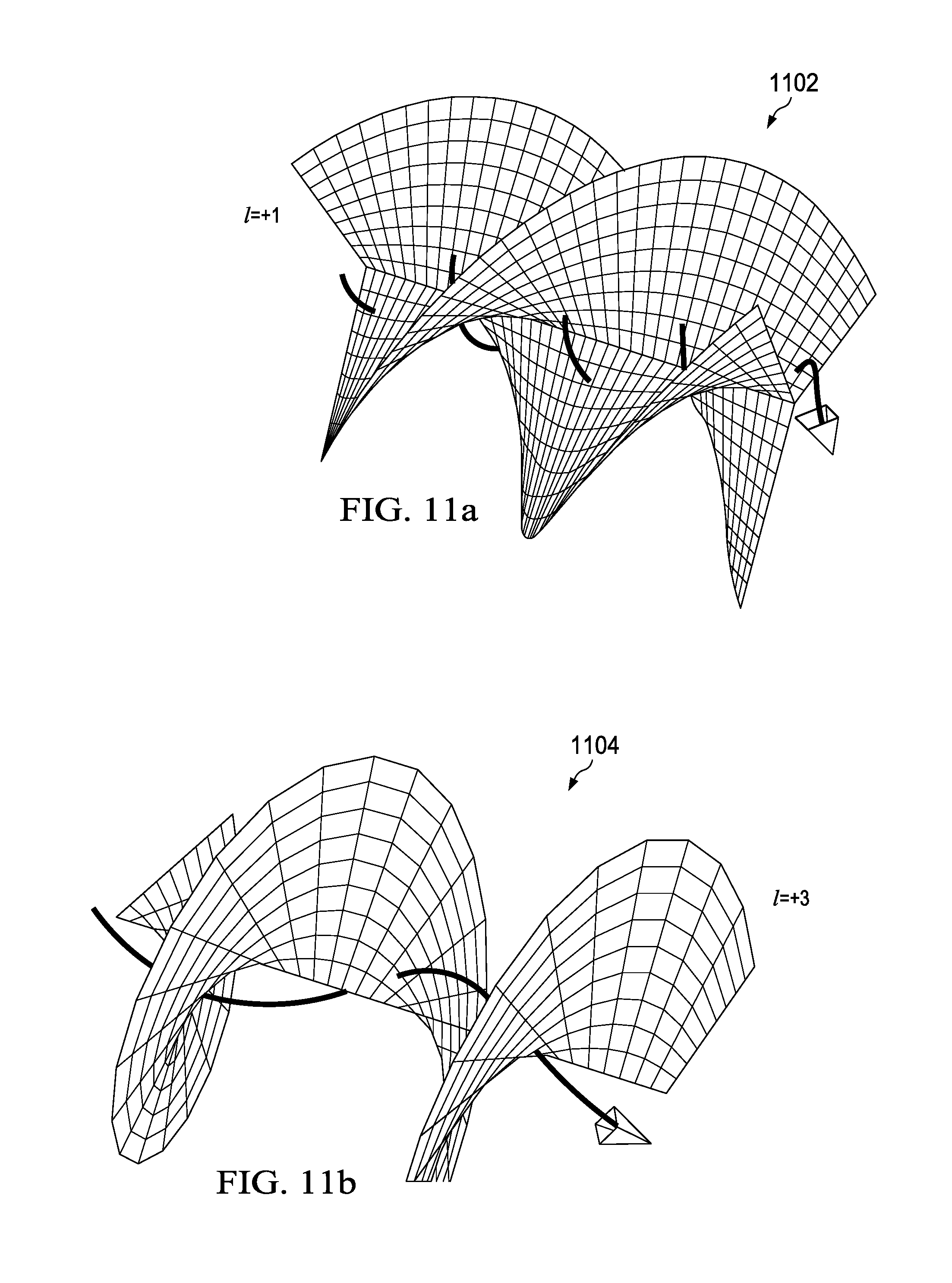
[0091] FIGS. 11A through 11C illustrate the differences in signals having different helicity (i.e., orbital angular momentums). Each of the spiraling Poynting vectors associated with the signals 1102, 1104, and 1106 provide a different shaped signal. Signal 1102 has an orbital angular momentum of +1, signal 1104 has an orbital angular momentum of +3, and signal 1106 has an orbital angular momentum of -4. Each signal has a distinct angular momentum and associated Poynting vector enabling the signal to be distinguished from other signals within a same frequency. This allows differing type of information to be transmitted on the same frequency, since these signals are separately detectable and do not interfere with each other (Eigen channels).
[0092] FIG. 11D illustrates the propagation of Poynting vectors for various Eigen modes. Each of the rings 1120 represents a different Eigen mode or twist representing a different orbital angular momentum within the same frequency. Each of these rings 1120 represents a different orthogonal channel. Each of the Eigen modes has a Poynting vector 1122 associated therewith.
[0093] Topological charge may be multiplexed to the frequency for either linear or circular polarization. In case of linear polarizations, topological charge would be multiplexed on vertical and horizontal polarization. In case of circular polarization, topological charge would multiplex on left hand and right hand circular polarizations. The topological charge is another name for the helicity index "I" or the amount of twist or OAM applied to the signal. The helicity index may be positive or negative. In RF, different topological charges can be created and muxed together and de-muxed to separate the topological charges.
[0094] The topological charges s can be created using Spiral Phase Plates (SPPs) as shown in FIG. 11E using a proper material with specific index of refraction and ability to machine shop or phase mask, holograms created of new materials or a new technique to create an RF version of Spatial Light Modulator (SLM) that does the twist of the RF waves (as opposed to optical beams) by adjusting voltages on the device resulting in twisting of the RF waves with a specific topological charge. Spiral Phase plates can transform a RF plane wave (=0) to a twisted RF wave of a specific helicity (i.e. =+1).
[0095] Cross talk and multipath interference can be corrected using RF Multiple-Input-Multiple-Output (MIMO). Most of the channel impairments can be detected using a control or pilot channel and be corrected using algorithmic techniques (closed loop control system).
[0096] As described previously with respect to FIG. 5, each of the multiple data streams applied within the processing circuitry has a multiple layer overlay modulation scheme applied thereto.
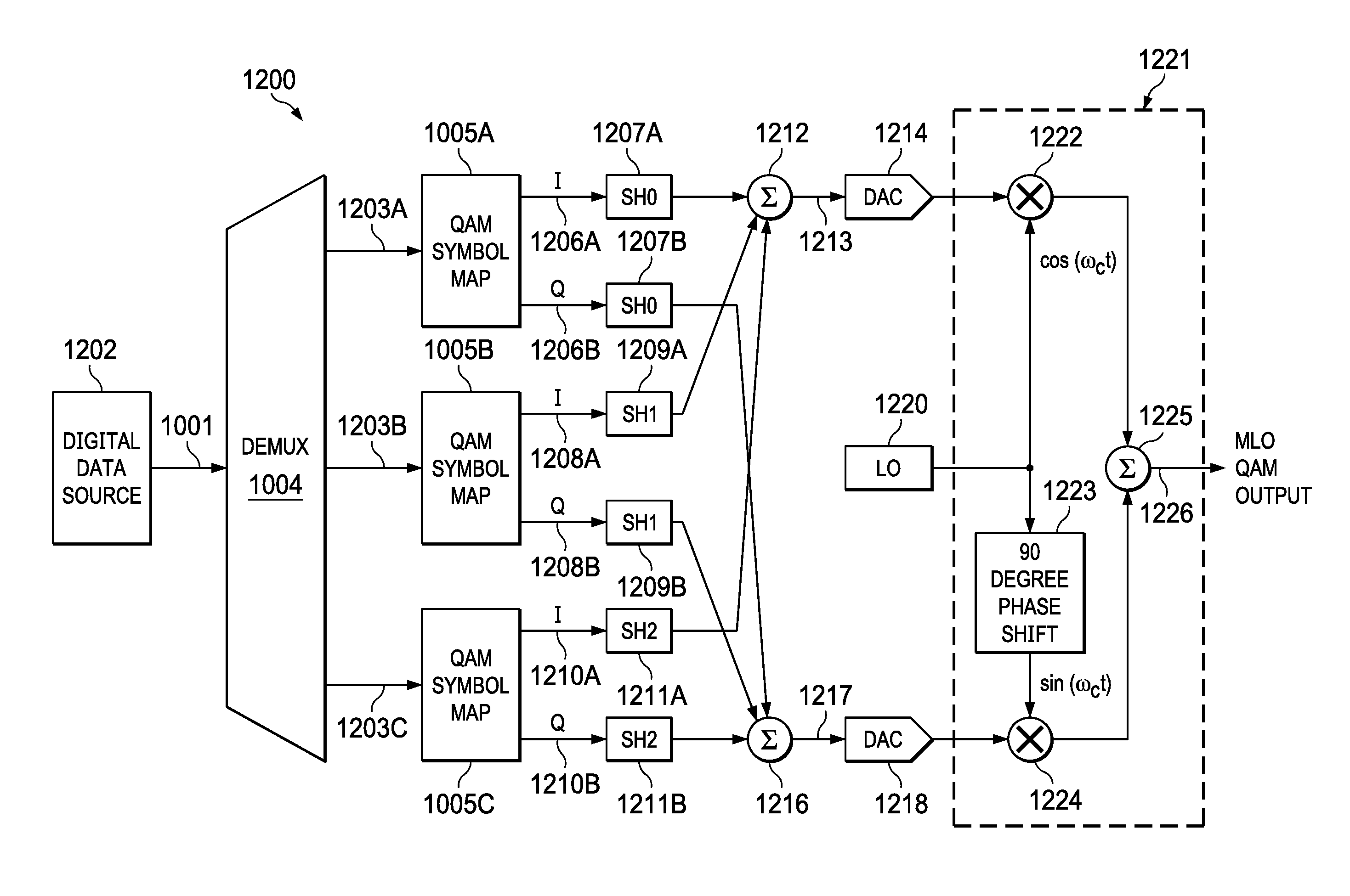
[0097] Referring now to FIG. 12, the reference number 1200 generally indicates an embodiment of a multiple level overlay (MLO)/quantum level overlay (QLO) modulation system, although it should be understood that the term MLO and the illustrated system 1200 are examples of embodiments. The MLO/QLO system may comprise one such as that disclosed in U.S. Pat. No. 8,503,546 entitled Multiple Layer Overlay Modulation which is incorporated herein by reference. In one example, the modulation system 1200 would be implemented within the multiple level overlay modulation box 504 of FIG. 5. System 1200 takes as input an input data stream 1201 from a digital source 1202, which is separated into three parallel, separate data streams, 1203A-1203C, of logical 1s and 0s by input stage demultiplexer (DEMUX) 1004. Data stream 1001 may represent a data file to be transferred, or an audio or video data stream. It should be understood that a greater or lesser number of separated data streams may be used. In some of the embodiments, each of the separated data streams 1203A-1203C has a data rate of 1/N of the original rate, where N is the number of parallel data streams. In the embodiment illustrated in FIG. 12, N is 3.
[0098] Each of the separated data streams 1203A-1203C is mapped to a quadrature amplitude modulation (QAM) symbol in an M-QAM constellation, for example, 16 QAM or 64 QAM, by one of the QAM symbol mappers 1205A-C. The QAM symbol mappers 1205A-C are coupled to respective outputs of DEMUX 1204, and produced parallel in phase (I) 1206A, 1208A, and 1210A and quadrature phase (Q) 1206B, 1208B, and 1210B data streams at discrete levels. For example, in 64 QAM, each I and Q channel uses 8 discrete levels to transmit 3 bits per symbol. Each of the three I and Q pairs, 1206A-1206B, 1208A-1208B, and 1210A-1210B, is used to weight the output of the corresponding pair of function generators 1207A-1207B, 1209A-1209B, and 1211A-1211B, which in some embodiments generate signals such as the modified Hermite polynomials described above and weights them based on the amplitude value of the input symbols. This provides 2N weighted or modulated signals, each carrying a portion of the data originally from income data stream 1201, and is in place of modulating each symbol in the I and Q pairs, 1206A-1206B, 1208A-1208B, and 1210A-1210B with a raised cosine filter, as would be done for a prior art QAM system. In the illustrated embodiment, three signals are used, SH0, SH1, and SH2, which correspond to modifications of H0, H1, and H2, respectively, although it should be understood that different signals may be used in other embodiments.
[0099] The weighted signals are not subcarriers, but rather are sublayers of a modulated carrier, and are combined, superimposed in both frequency and time, using summers 1212 and 1216, without mutual interference in each of the I and Q dimensions, due to the signal orthogonality. Summers 1212 and 1216 act as signal combiners to produce composite signals 1213 and 1217. The weighted orthogonal signals are used for both I and Q channels, which have been processed equivalently by system 1200, and are summed before the QAM signal is transmitted. Therefore, although new orthogonal functions are used, some embodiments additionally use QAM for transmission. Because of the tapering of the signals in the time domain, as will be shown in FIGS. 16A through 16K, the time domain waveform of the weighted signals will be confined to the duration of the symbols. Further, because of the tapering of the special signals and frequency domain, the signal will also be confined to frequency domain, minimizing interface with signals and adjacent channels.
[0100] The composite signals 1213 and 1217 are converted to analogue signals 1215 and 1219 using digital to analogue converters 1214 and 1218, and are then used to modulate a carrier signal at the frequency of local oscillator (LO) 1220, using modulator 1221. Modulator 1221 comprises mixers 1222 and 1224 coupled to DACs 1214 and 1218, respectively. Ninety degree phase shifter 1223 converts the signals from LO 1220 into a Q component of the carrier signal. The output of mixers 1222 and 1224 are summed in summer 1225 to produce output signals 1226.
[0101] MLO/QLO can be used with a variety of transport mediums, such as wire, optical, and wireless, and may be used in conjunction with QAM. This is because MLO/QLO uses spectral overlay of various signals, rather than spectral overlap. Bandwidth utilization efficiency may be increased by an order of magnitude, through extensions of available spectral resources into multiple layers. The number of orthogonal signals is increased from 2, cosine and sine, in the prior art, to a number limited by the accuracy and jitter limits of generators used to produce the orthogonal polynomials. In this manner, MLO/QLO extends each of the I and Q dimensions of QAM to any multiple access techniques such as GSM, code division multiple access (CDMA), wide band CDMA (WCDMA), high speed downlink packet access (HSPDA), evolution-data optimized (EV-DO), orthogonal frequency division multiplexing (OFDM), world-wide interoperability for microwave access (WIMAX), and long term evolution (LTE) systems. MLO/QLO may be further used in conjunction with other multiple access (MA) schemes such as frequency division duplexing (FDD), time division duplexing (TDD), frequency division multiple access (FDMA), and time division multiple access (TDMA). Overlaying individual orthogonal signals over the same frequency band allows creation of a virtual bandwidth wider than the physical bandwidth, thus adding a new dimension to signal processing. This modulation is applicable to twisted pair, cable, fiber optic, satellite, broadcast, free-space optics, and all types of wireless access. The method and system are compatible with many current and future multiple access systems, including EV-DO, UMB, WIMAX, WCDMA (with or without), multimedia broadcast multicast service (MBMS)/multiple input multiple output (MIMO), HSPA evolution, and LTE.
[0102] Referring now to FIG. 13, an MLO/QLO demodulator 1300 is illustrated, although it should be understood that the term MLO/QLO and the illustrated system 1300 are examples of embodiments. The modulator 1300 takes as input an MLO/QLO signal 1126 which may be similar to output signal 1226 from system 1200. Synchronizer 1327 extracts phase information, which is input to local oscillator 1320 to maintain coherence so that the modulator 1321 can produce base band to analogue I signal 1315 and Q signal 1319. The modulator 1321 comprises mixers 1322 and 1324, which, coupled to OL 1320 through 90 degree phase shifter 1323. I signal 1315 is input to each of signal filters 1307A, 1309A, and 1311A, and Q signal 1319 is input to each of signal filters 1307B, 1309B, and 1311B. Since the orthogonal functions are known, they can be separated using correlation or other techniques to recover the modulated data. Information in each of the I and Q signals 1315 and 1319 can be extracted from the overlapped functions which have been summed within each of the symbols because the functions are orthogonal in a correlative sense.
[0103] In some embodiments, signal filters 1307A-1307B, 1309A-1309B, and 1311A-1311B use locally generated replicas of the polynomials as known signals in match filters. The outputs of the match filters are the recovered data bits, for example, equivalence of the QAM symbols 1306A-1306B, 1308A-1308B, and 1310A-1310B of system 1300. Signal filters 1307A-1307B, 1309A-1309B, and 1311A-1311B produce 2n streams of n, I, and Q signal pairs, which are input into demodulators 1328-1333. Demodulators 1328-1333 integrate the energy in their respective input signals to determine the value of the QAM symbol, and hence the logical 1s and 0s data bit stream segment represented by the determined symbol. The outputs of the modulators 1328-1333 are then input into multiplexers (MUXs) 1305A-1305C to generate data streams 1303A-1303C. If system 1300 is demodulating a signal from system 1200, data streams 1303A-1303C correspond to data streams 1203A-1203C. Data streams 1303A-1303C are multiplexed by MUX 1304 to generate data output stream 1301. In summary, MLO/QLO signals are overlayed (stacked) on top of one another on transmitter and separated on receiver.
[0104] MLO/QLO may be differentiated from CDMA or OFDM by the manner in which orthogonality among signals is achieved. MLO/QLO signals are mutually orthogonal in both time and frequency domains, and can be overlaid in the same symbol time bandwidth product. Orthogonality is attained by the correlation properties, for example, by least sum of squares, of the overlaid signals. In comparison, CDMA uses orthogonal interleaving or displacement of signals in the time domain, whereas OFDM uses orthogonal displacement of signals in the frequency domain.
[0105] Bandwidth efficiency may be increased for a channel by assigning the same channel to multiple users. This is feasible if individual user information is mapped to special orthogonal functions. CDMA systems overlap multiple user information and views time intersymbol orthogonal code sequences to distinguish individual users, and OFDM assigns unique signals to each user, but which are not overlaid, are only orthogonal in the frequency domain. Neither CDMA nor OFDM increases bandwidth efficiency. CDMA uses more bandwidth than is necessary to transmit data when the signal has a low signal to noise ratio (SNR). OFDM spreads data over many subcarriers to achieve superior performance in multipath radiofrequency environments. OFDM uses a cyclic prefix OFDM to mitigate multipath effects and a guard time to minimize intersymbol interference (ISI), and each channel is mechanistically made to behave as if the transmitted waveform is orthogonal. (Sync function for each subcarrier in frequency domain.)
[0106] In contrast, MLO/QLO uses a set of functions which effectively form an alphabet that provides more usable channels in the same bandwidth, thereby enabling high bandwidth efficiency. Some embodiments of MLO/QLO do not require the use of cyclic prefixes or guard times, and therefore, outperforms OFDM in spectral efficiency, peak to average power ratio, power consumption, and requires fewer operations per bit. In addition, embodiments of MLO/QLO are more tolerant of amplifier nonlinearities than are CDMA and OFDM systems.
[0107] FIG. 14 illustrates an embodiment of an MLO/QLO transmitter system 1400, which receives input data stream 1401. System 1400 represents a modulator/controller 1401, which incorporates equivalent functionality of DEMUX 1204, QAM symbol mappers 1205A-C, function generators 1207A-1207B, 1209A-1209B, and 1211A-1211B, and summers 1212 and 1216 of system 1200, shown in FIG. 12. However, it should be understood that modulator/controller 1401 may use a greater or lesser quantity of signals than the three illustrated in system 1200. Modulator/controller 1401 may comprise an application specific integrated circuit (ASIC), a field programmable gate array (FPGA), and/or other components, whether discrete circuit elements or integrated into a single integrated circuit (IC) chip.
[0108] Modulator/controller 1401 is coupled to DACs 1404 and 1407, communicating a 10 bit I signal 1402 and a 10 bit Q signal 1405, respectively. In some embodiments, I signal 1402 and Q signal 1405 correspond to composite signals 1213 and 1217 of system 1200. It should be understood, however, that the 10 bit capacity of I signal 1402 and Q signal 1405 is merely representative of an embodiment. As illustrated, modulator/controller 1401 also controls DACs 1404 and 1407 using control signals 1403 and 1406, respectively. In some embodiments, DACs 1404 and 1407 each comprise an AD5433, complementary metal oxide semiconductor (CMOS) 10 bit current output DAC. In some embodiments, multiple control signals are sent to each of DACs 1404 and 1407.
[0109] DACs 1404 and 1407 output analogue signals 1215 and 1219 to quadrature modulator 1221, which is coupled to LO 1220. The output of modulator 1220 is illustrated as coupled to a transmitter 1408 to transmit data wirelessly, although in some embodiments, modulator 1221 may be coupled to a fiber-optic modem, a twisted pair, a coaxial cable, or other suitable transmission media.
[0110] FIG. 15 illustrates an embodiment of an MLO/QLO receiver system 1500 capable of receiving and demodulating signals from system 1400. System 1500 receives an input signal from a receiver 1508 that may comprise input medium, such as RF, wired or optical. The modulator 1321 driven by LO 1320 converts the input to baseband I signal 1315 and Q signal 1319. I signal 1315 and Q signal 1319 are input to analogue to digital converter (ADC) 1509.
[0111] ADC 1509 outputs 10 bit signal 1510 to demodulator/controller 1501 and receives a control signal 1512 from demodulator/controller 1501. Demodulator/controller 1501 may comprise an application specific integrated circuit (ASIC), a field programmable gate array (FPGA), and/or other components, whether discrete circuit elements or integrated into a single integrated circuit (IC) chip. Demodulator/controller 1501 correlates received signals with locally generated replicas of the signal set used, in order to perform demodulation and identify the symbols sent. Demodulator/controller 1501 also estimates frequency errors and recovers the data clock, which is used to read data from the ADC 1509. The clock timing is sent back to ADC 1509 using control signal 1512, enabling ADC 1509 to segment the digital I and Q signals 1315 and 1319. In some embodiments, multiple control signals are sent by demodulator/controller 1501 to ADC 1509. Demodulator/controller 1501 also outputs data signal 1301.
[0112] Hermite polynomials are a classical orthogonal polynomial sequence, which are the Eigenstates of a quantum harmonic oscillator. Signals based on Hermite polynomials possess the minimal time-bandwidth product property described above, and may be used for embodiments of MLO/QLO systems. However, it should be understood that other signals may also be used, for example orthogonal polynomials such as Jacobi polynomials, Gegenbauer polynomials, Legendre polynomials, Chebyshev polynomials, and Laguerre polynomials. Q-functions are another class of functions that can be employed as a basis for MLO/QLO signals.
[0113] In quantum mechanics, a coherent state is a state of a quantum harmonic oscillator whose dynamics most closely resemble the oscillating behavior of a classical harmonic oscillator system. A squeezed coherent state is any state of the quantum mechanical Hilbert space, such that the uncertainty principle is saturated. That is, the product of the corresponding two operators takes on its minimum value. In embodiments of an MLO/QLO system, operators correspond to time and frequency domains wherein the time-bandwidth product of the signals is minimized. The squeezing property of the signals allows scaling in time and frequency domain simultaneously, without losing mutual orthogonality among the signals in each layer. This property enables flexible implementations of MLO/QLO systems in various communications systems.
[0114] Because signals with different orders are mutually orthogonal, they can be overlaid to increase the spectral efficiency of a communication channel. For example, when n=0, the optimal baseband signal will have a time-bandwidth product of 1/2, which is the Nyquist Inter-Symbol Interference (ISI) criteria for avoiding ISI. However, signals with time-bandwidth products of 3/2, 5/2, 7/2, and higher, can be overlaid to increase spectral efficiency.
[0115] An embodiment of an MLO/QLO system uses functions based on modified Hermite polynomials, 4n, and are defined by:
.psi. n ( t , .xi. ) = ( tanh .xi. ) n / 2 2 n / 2 ( n ! cosh .xi. ) 1 / 2 e 1 2 t 2 [ 1 - ta nh .xi. ] H n ( t 2 cosh .xi. sinh .xi. ) ##EQU00009##
where t is time, and .xi. is a bandwidth utilization parameter. Plots of .PSI..sub.n for n ranging from 0 to 9, along with their Fourier transforms (amplitude squared), are shown in FIGS. 5A-5K. The orthogonality of different orders of the functions may be verified by integrating:
.intg..intg..psi..sub.n(t,.xi.).psi..sub.m(t,.xi.)dtd.xi.
[0116] The Hermite polynomial is defined by the contour integral:
H n ( z ) = n ! 2 .pi. i e - t 2 + 2 t 2 t - n - 1 dt , ##EQU00010##
where the contour encloses the origin and is traversed in a counterclockwise direction. Hermite polynomials are described in Mathematical Methods for Physicists, by George Arfken, for example on page 416, the disclosure of which is incorporated by reference.
[0117] FIGS. 16A-16K illustrate representative MLO/QLO signals and their respective spectral power densities based on the modified Hermite polynomials .PSI..sub.0 for n ranging from 0 to 9. FIG. 16A shows plots 1601 and 1604. Plot 1601 comprises a curve 1627 representing .PSI..sub.0 plotted against a time axis 1602 and an amplitude axis 1603. As can be seen in plot 1601, curve 1627 approximates a Gaussian curve. Plot 1604 comprises a curve 1637 representing the power spectrum of .PSI..sub.0 plotted against a frequency axis 1605 and a power axis 1606. As can be seen in plot 1604, curve 1637 also approximates a Gaussian curve. Frequency domain curve 1607 is generated using a Fourier transform of time domain curve 1627. The units of time and frequency on axis 1602 and 1605 are normalized for baseband analysis, although it should be understood that since the time and frequency units are related by the Fourier transform, a desired time or frequency span in one domain dictates the units of the corresponding curve in the other domain. For example, various embodiments of MLO/QLO systems may communicate using symbol rates in the megahertz (MHz) or gigahertz (GHz) ranges and the non-0 duration of a symbol represented by curve 1627, i.e., the time period at which curve 1627 is above 0 would be compressed to the appropriate length calculated using the inverse of the desired symbol rate. For an available bandwidth in the megahertz range, the non-0 duration of a time domain signal will be in the microsecond range.
[0118] FIGS. 16B-16J show plots 1607-1624, with time domain curves 1628-1636 representing .PSI..sub.1 through .PSI..sub.9, respectively, and their corresponding frequency domain curves 1638-1646. As can be seen in FIGS. 16A-16J, the number of peaks in the time domain plots, whether positive or negative, corresponds to the number of peaks in the corresponding frequency domain plot. For example, in plot 1623 of FIG. 16J, time domain curve 1636 has five positive and five negative peaks. In corresponding plot 1624 therefore, frequency domain curve 1646 has ten peaks.
[0119] FIG. 16K shows overlay plots 1625 and 1626, which overlay curves 1627-1636 and 1637-1646, respectively. As indicated in plot 1625, the various time domain curves have different durations. However, in some embodiments, the non-zero durations of the time domain curves are of similar lengths. For an MLO/QLO system, the number of signals used represents the number of overlays and the improvement in spectral efficiency. It should be understood that, while ten signals are disclosed in FIGS. 16A-16K, a greater or lesser quantity of signals may be used, and that further, a different set of signals, rather than the .PSI..sub.n signals plotted, may be used.
[0120] MLO/QLO signals used in a modulation layer have minimum time-bandwidth products, which enable improvements in spectral efficiency, and are quadratically integrable. This is accomplished by overlaying multiple demultiplexed parallel data streams, transmitting them simultaneously within the same bandwidth. The key to successful separation of the overlaid data streams at the receiver is that the signals used within each symbols period are mutually orthogonal. MLO/QLO overlays orthogonal signals within a single symbol period. This orthogonality prevents ISI and inter-carrier interference (ICI).
[0121] Because MLO/QLO works in the baseband layer of signal processing, and some embodiments use QAM architecture, conventional wireless techniques for optimizing air interface, or wireless segments, to other layers of the protocol stack will also work with MLO/QLO. Techniques such as channel diversity, equalization, error correction coding, spread spectrum, interleaving and space-time encoding are applicable to MLO/QLO. For example, time diversity using a multipath-mitigating rake receiver can also be used with MLO/QLO. MLO/QLO provides an alternative for higher order QAM, when channel conditions are only suitable for low order QAM, such as in fading channels. MLO/QLO can also be used with CDMA to extend the number of orthogonal channels by overcoming the Walsh code limitation of CDMA. MLO/QLO can also be applied to each tone in an OFDM signal to increase the spectral efficiency of the OFDM systems.
[0122] Embodiments of MLO/QLO systems amplitude modulate a symbol envelope to create sub-envelopes, rather than sub-carriers. For data encoding, each sub-envelope is independently modulated according to N-QAM, resulting in each sub-envelope independently carrying information, unlike OFDM. Rather than spreading information over many sub-carriers, as is done in OFDM, for MLO/QLO, each sub-envelope of the carrier carries separate information. This information can be recovered due to the orthogonality of the sub-envelopes defined with respect to the sum of squares over their duration and/or spectrum. Pulse train synchronization or temporal code synchronization, as needed for CDMA, is not an issue, because MLO/QLO is transparent beyond the symbol level. MLO/QLO addresses modification of the symbol, but since CDMA and TDMA are spreading techniques of multiple symbol sequences over time. MLO/QLO can be used along with CDMA and TDMA. The signals created from the minimization of the time-bandwidth products can be used in temporal modulation.
[0123] FIG. 17 illustrates a comparison of MLO/QLO signal widths in the time and frequency domains. Time domain envelope representations 1701-1703 of signals SH0-SH3 are illustrated as all having a duration T.sub.S. SH0-SH3 may represent PSI.sub.0-PSI.sub.2, or may be other signals. The corresponding frequency domain envelope representations are 1705-1707, respectively. SH0 has a bandwidth BW, SH1 has a bandwidth three times BW, and SH2 has a bandwidth of 5BW, which is five times as great as that of SH0. The bandwidth used by an MLO/QLO system will be determined, at least in part, by the widest bandwidth of any of the signals used. If each layer uses only a single signal type within identical time windows, the spectrum will not be fully utilized, because the lower order signals will use less of the available bandwidth than is used by the higher order signals.
[0124] FIG. 18 illustrates a spectral alignment of MLO/QLO signals that accounts for the differing bandwidths of the signals, and makes spectral usage more uniform, using SH0-SH3. Blocks 1801-1804 are frequency domain blocks of an OFDM signal with multiple subcarriers. Block 1803 is expanded to show further detail. Block 1803 comprises a first layer 1803x comprised of multiple SH0 envelopes 1803a-1803o. A second layer 1803y of SH1 envelopes 1803p-1803t has one third the number of envelopes as the first layer. In the illustrated example, first layer 1803x has 15 SH0 envelopes, and second layer 1803y has five SH1 envelopes. This is because, since the SH1 bandwidth envelope is three times as wide as that of SH0, 15 SH0 envelopes occupy the same spectral width as five SH1 envelopes. The third layer 1803z of block 1803 comprises three SH2 envelopes 1803u-1803w, because the SH2 envelope is five times the width of the SH0 envelope.
[0125] The total required bandwidth for such an implementation is a multiple of the least common multiple of the bandwidths of the MLO/QLO signals. In the illustrated example, the least common multiple of the bandwidth required for SH0, SH1, and SH2 is 15BW, which is a block in the frequency domain. The OFDM-MLO/QLO signal can have multiple blocks, and the spectral efficiency of this illustrated implementation is proportional to (15+5+3)/15.
[0126] FIG. 19 illustrates another spectral alignment of MLO/QLO signals, which may be used alternatively to alignment scheme shown in FIG. 18. In the embodiment illustrated in FIG. 19, the OFDM-MLO/QLO implementation stacks the spectrum of SH0, SH1, and SH2 in such a way that the spectrum in each layer is utilized uniformly. Layer 1900A comprises envelopes 1901A-1901D, which includes both SH0 and SH2 envelopes. Similarly, layer 1900C, comprising envelopes 1903A-1903D, includes both SH0 and SH2 envelopes. Layer 1900B, however, comprising envelopes 1902A-1902D, includes only SH1 envelopes. Using the ratio of envelope sizes described above, it can be easily seen that BW+5BW=3BW+3BW. Thus, for each SH0 envelope in layer 1900A, there is one SH2 envelope also in layer 1900C and two SH1 envelopes in layer 1900B.
Three Scenarios Compared:
[0127] 1) MLO/QLO with 3 Layers defined by:
.intg. 0 ( t ) = W 0 e - t 2 4 , W 0 = 0.6316 ##EQU00011## .intg. 0 ( t ) = W 1 t e - t 2 4 , W 1 .apprxeq. 0.6316 ##EQU00011.2## .intg. 0 ( t ) = W 2 ( t 2 - 1 ) e - t 2 4 , W 2 .apprxeq. 0.6316 ##EQU00011.3##
(The current FPGA implementation uses the truncation interval of [-6, 6].) 2) Conventional scheme using rectangular pulse 3) Conventional scheme using a square-root raised cosine (SRRC) pulse with a roll-off factor of 0.5
[0128] For MLO/QLO pulses and SRRC pulse, the truncation interval is denoted by [-t1, t1] in the following figures. For simplicity, we used the MLO/QLO pulses defined above, which can be easily scaled in time to get the desired time interval (say micro-seconds or nano-seconds). For the SRRC pulse, we fix the truncation interval of [-3T, 3T] where T is the symbol duration for all results presented in this document.
Bandwidth Efficiency
[0129] The X-dB bounded power spectral density bandwidth is defined as the smallest frequency interval outside which the power spectral density (PSD) is X dB below the maximum value of the PSD. The X-dB can be considered as the out-of-band attenuation.
[0130] The bandwidth efficiency is expressed in Symbols per second per Hertz. The bit per second per Hertz can be obtained by multiplying the symbols per second per Hertz with the number of bits per symbol (i.e., multiplying with log 2 M for M-ary QAM).
[0131] Truncation of MLO/QLO pulses introduces inter-layer interferences (ILI). However, the truncation interval of [-6, 6] yields negligible ILI while [-4, 4] causes slight tolerable ILI.
[0132] The bandwidth efficiency of MLO/QLO may be enhanced by allowing inter-symbol interference (ISI). To realize this enhancement, designing transmitter side parameters as well as developing receiver side detection algorithms and error performance evaluation can be performed.
[0133] Referring now to FIG. 20, there is illustrated the power spectral density of each layer SH0-SH2 within MLO/QLO and also for the combined three layer MLO/QLO. 2002 illustrates the power spectral density of the SH0 layer; 2004 illustrates the power spectral density of the SH1 layer; 2006 illustrates the power spectral density of the SH2 layer, and 2008 illustrates the combined power spectral density of each layer.
[0134] Referring now to FIG. 21, there is illustrated the power spectral density of each layer as well as the power spectral density of the combined three layer in a log scale. 2102 represents the SH0 layer. 2104 represents the SH1 layer. 2106 represents the SH2 layer. 2108 represents the combined layers.
[0135] Referring now to FIG. 22, there is a bandwidth efficiency comparison versus out of band attenuation (X-dB) where quantum level overlay pulse truncation interval is [-6,6] and the symbol rate is 1/6. Referring also to FIG. 23, there is illustrated the bandwidth efficiency comparison versus out of band attenuation (X-dB) where quantum level overlay pulse truncation interval is [-6,6] and the symbol rate is 1/4.
[0136] The QLO signals are generated from the Physicist's special Hermite functions:
f n ( t , .alpha. ) = .alpha. .pi. n ! 2 n H n ( .alpha. t ) e - .alpha. 2 t 2 2 , .alpha. > 0 ##EQU00012##
[0137] Note that the initial hardware implementation is using
.alpha. = 1 2 ##EQU00013##
and for consistency with his part,
.alpha. = 1 2 ##EQU00014##
is used in all figures related to the spectral efficiency.
[0138] Let the low-pass-equivalent power spectral density (PSD) of the combined QLO signals be X(f) and its bandwidth be B. Here the bandwidth is defined by one of the following criteria.
ACLR1 (First Adjacent Channel Leakage Ratio) in dBc Equals:
[0139] ACLR 1 = .intg. B / 2 3 B / 2 X ( f ) df .intg. - .infin. .infin. X ( f ) df ##EQU00015##
ACLR2 (Second Adjacent Channel Leakage Ratio) in dBc Equals:
[0140] ACLR 2 = .intg. 3 B / 2 5 B / 2 X ( f ) df .intg. - .infin. .infin. X ( f ) df ##EQU00016##
Out-of-Band Power to Total Power Ratio is:
[0141] 2 .intg. B / 2 .infin. X ( f ) df .intg. - .infin. .infin. X ( f ) df ##EQU00017##
The Band-Edge PSD in dBc/100 kHz Equals:
.intg. B / 2 B 2 + 10 5 X ( f ) df .intg. - .infin. .infin. X ( f ) df ##EQU00018##
[0142] Referring now to FIG. 24 there is illustrated a performance comparison using ACLR1 and ACLR2 for both a square root raised cosine scheme and a multiple layer overlay scheme. Line 2402 illustrates the performance of a square root raised cosine 2402 using ACLR1 versus an MLO/QLO 2404 using ACLR1. Additionally, a comparison between a square root raised cosine 2406 using ACLR2 versus MLO/QLO 2408 using ACLR2 is illustrated. Table A illustrates the performance comparison using ACLR.
TABLE-US-00001 TABLE A Criteria: ACLR1 .ltoreq.-30 dBc per bandwidth Spectral Efficiency ACLR .ltoreq.-43 dBc per bandwidth (Symbol/sec/Hz) Gain SRRC [-8T, 8T] = 0.22 0.8765 1.0 QLO N Layers Symbol Duration [Tmol] [-8, 8] N = 3 Tmol = 4 1.133 1.2926 N = 4 Tmol = 5 1.094 1.2481 Tmol = 4 1.367 1.5596 N = 10 Tmol = 8 1.185 1.3520 Tmol = 7 1.355 1.5459 Tmol = 6 1.580 1.8026 Tmol = 5 1.896 2.1631 Tmol = 4 2.371 2.7051
[0143] Referring now to FIG. 25, there is illustrated a performance comparison between a square root raised cosine 2502 and a MLO/QLO 2504 using out-of-band power. Referring now also to Table B, there is illustrated a more detailed comparison of the performance using out-of-band power.
TABLE-US-00002 TABLE B Table 3: Performance Comparison Using Out-of-Band Power Criterion: Spectral Efficiency Out-of-band Power/Total .ltoreq.-30 dB (Symbol/sec/Hz) Gain SRRC [-8T, 8T] = 0.22 0.861 1.0 QLO N Layers Symbol Duration [Tmol] [-8, 8] N = 3 Tmol = 4 1.080 1.2544 N = 4 Tmol = 5 1.049 1.2181 Tmol = 4 1.311 1.5226 N = 10 Tmol = 8 1.152 1.3380 Tmol = 7 1.317 1.5296 Tmol = 6 1.536 1.7840 Tmol = 5 1.844 2.1417 Tmol = 4 2.305 2.6771
[0144] Referring now to FIG. 26, there is further provided a performance comparison between a square root raised cosine 2602 and a MLO/QLO 2604 using band-edge PSD. A more detailed illustration of the performance comparison is provided in Table C.
TABLE-US-00003 TABLE C Table: 4 Performance Comparison Using Band-Edge PSD Criterion: Spectral Efficiency Band-Edge PSD = -50 dBc/100 kHz (Symbol/sec/Hz) Gain SRRC [-8T, 8T] = 0.22 0.810 1.0 QLO N Layers Symbol Duration [Tmol] [-8, 8] N = 3 Tmol = 4 0.925 1.1420 N = 4 Tmol = 5 0.912 1.1259 Tmol = 4 1.14 1.4074 N = 10 Tmol = 8 1.049 1.2951 Tmol = 7 1.198 1.4790 Tmol = 6 1.398 1.7259 Tmol = 5 1.678 2.0716 Tmol = 4 2.097 2.5889
[0145] Referring now to FIGS. 27 and 28, there are more particularly illustrated the transmit subsystem (FIG. 27) and the receiver subsystem (FIG. 28). The transceiver is realized using basic building blocks available as Commercially Off The Shelf products. Modulation, demodulation and Special Hermite correlation and de-correlation are implemented on a FPGA board. The FPGA board 2802 at the receiver 2800 estimated the frequency error and recovers the data clock (as well as data), which is used to read data from the analog-to-digital (ADC) board 2806. The FGBA board 2800 also segments the digital I and Q channels.
[0146] On the transmitter side 2700, the FPGA board 2702 realizes the special hermite correlated QAM signal as well as the necessary control signals to control the digital-to-analog (DAC) boards 2704 to produce analog I&Q baseband channels for the subsequent up conversion within the direct conversion quad modulator 2706. The direct conversion quad modulator 2706 receives an oscillator signal from oscillator 2708.
[0147] The ADC 2806 receives the I&Q signals from the quad demodulator 2808 that receives an oscillator signal from 2810.
[0148] Neither power amplifier in the transmitter nor an LNA in the receiver is used since the communication will take place over a short distance. The frequency band of 2.4-2.5 GHz (ISM band) is selected, but any frequency band of interest may be utilized.
[0149] MIMO uses diversity to achieve some incremental spectral efficiency. Each of the signals from the antennas acts as an independent orthogonal channel. With QLO, the gain in spectral efficiency comes from within the symbol and each QLO signal acts as independent channels as they are all orthogonal to one another in any permutation. However, since QLO is implemented at the bottom of the protocol stack (physical layer), any technologies at higher levels of the protocol (i.e. Transport) will work with QLO. Therefore one can use all the conventional techniques with QLO. This includes RAKE receivers and equalizers to combat fading, cyclical prefix insertion to combat time dispersion and all other techniques using beam forming and MIMO to increase spectral efficiency even further.
[0150] When considering spectral efficiency of a practical wireless communication system, due to possibly different practical bandwidth definitions (and also not strictly bandlimited nature of actual transmit signal), the following approach would be more appropriate.
[0151] Referring now to FIG. 29, consider the equivalent discrete time system, and obtain the Shannon capacity for that system (will be denoted by Cd). Regarding the discrete time system, for example, for conventional QAM systems in AWGN, the system will be:
y[n]=ax[n]+w[n]
where a is a scalar representing channel gain and amplitude scaling, x[n] is the input signal (QAM symbol) with unit average energy (scaling is embedded in a), y[n] is the demodulator (matched filter) output symbol, and index n is the discrete time index.
[0152] The corresponding Shannon capacity is:
C.sub.d=log.sub.2(1+|a|.sup.2/.sigma..sup.2)
where .sigma.2 is the noise variance (in complex dimension) and |a|2/.sigma.2 is the SNR of the discrete time system.
[0153] Second, compute the bandwidth W based on the adopted bandwidth definition (e.g., bandwidth defined by -40 dBc out of band power). If the symbol duration corresponding to a sample in discrete time (or the time required to transmit C.sub.d bits) is T, then the spectral efficiency can be obtained as:
C/W=C.sub.d/(TW) bps/Hz
[0154] In discrete time system in AWGN channels, using Turbo or similar codes will give performance quite close to Shannon limit C.sub.d. This performance in discrete time domain will be the same regardless of the pulse shape used. For example, using either SRRC (square root raised cosine) pulse or a rectangle pulse gives the same C.sub.d (or C.sub.d/T). However, when we consider continuous time practical systems, the bandwidths of SRRC and the rectangle pulse will be different. For a typical practical bandwidth definition, the bandwidth for a SRRC pulse will be smaller than that for the rectangle pulse and hence SRRC will give better spectral efficiency. In other words, in discrete time system in AWGN channels, there is little room for improvement. However, in continuous time practical systems, there can be significant room for improvement in spectral efficiency.
[0155] Referring now to FIG. 30, there is illustrated a PSD plot (BLANK) of MLO/QLO, modified MLO/QLO (MMLO/QLO) and square root raised cosine (SRRC). From the illustration in FIG. 30, demonstrates the better localization property of MLO/QLO. An advantage of MLO/QLO is the bandwidth. FIG. 30 also illustrates the interferences to adjacent channels will be much smaller for MLO/QLO. This will provide additional advantages in managing, allocating or packaging spectral resources of several channels and systems, and further improvement in overall spectral efficiency. If the bandwidth is defined by the -40 dBc out of band power, the within-bandwidth PSDs of MLO/QLO and SRRC are illustrated in FIG. 31. The ratio of the bandwidths is about 1.536. Thus, there is significant room for improvement in spectral efficiency.
[0156] Modified MLO/QLO systems are based on block-processing wherein each block contains N MLO/QLO symbols and each MLO/QLO symbol has L layers. MMLO can be converted into parallel (virtual) orthogonal channels with different channel SNRs as illustrated in FIG. 32. The outputs provide equivalent discrete time parallel orthogonal channels of MMLO.
[0157] Note that the intersymbol interference caused pulse overlapping of MLO/QLO has been addressed by the parallel orthogonal channel conversion. As an example, the power gain of a parallel orthogonal virtual channel of MMLO with three layers and 40 symbols per block is illustrated in FIG. 33. FIG. 33 illustrates the channel power gain of the parallel orthogonal channels of MMLO with three layers and .PSI..sub.sim=3. By applying a water filling solution, an optimal power distribution across the orthogonal channels for a fixed transmit power may be obtained. The transmit power on the k.sup.th orthogonal channel is denoted by P.sub.k. Then the discrete time capacity of the MMLO can be given by:
C d + k = 1 k log 2 ( 1 + P k .alpha. k 2 .sigma. k 2 ) bits per block ##EQU00019##
Note that K depends on the number of MLO/QLO layers, the number of MLO/QLO symbols per block, and MLO/QLO symbol duration.
[0158] For MLO/QLO pulse duration defined by [-t.sub.1, t.sub.1], and symbol duration T.sub.mlo, the MMLO block length is:
T.sub.block=(N-1)T.sub.mlo+2t.sub.1
[0159] Suppose the bandwidth of MMLO signal based on the adopted bandwidth definition (ACLR, OBP, or other) is W.sub.mmlo, then the practical spectral efficiency of MMLO is given by:
C d W mmlo T block = 1 W mmlo { ( N - 1 ) T mlo + 2 t 1 ) } k = 1 K log 2 ( 1 + P k .alpha. k 2 .sigma. k 2 ) bps Hz ##EQU00020##
[0160] FIGS. 34-35 show the spectral efficiency comparison of MMLO with N=40 symbols per block, L=3 layers, T.sub.mlo=3, t.sub.1=8, and SRRC with duration [-8T, 8T], T=1, and the roll-off factor .beta.=0.22, at SNR of 5 dB. Two bandwidth definitions based on ACLR1 (first adjacent channel leakage power ratio) and OBP (out of band power) are used.
[0161] FIGS. 36-37 show the spectral efficiency comparison of MMLO with L=4 layers. The spectral efficiencies and the gains of MMLO for specific bandwidth definitions are shown in the following tables.
TABLE-US-00004 TABLE D Spectral Efficiency (bps/Hz) Gain with based on ACLR1 .ltoreq.30 dBc reference per bandwidth to SRRC SRRC 1.7859 1 MMLO (3 layers, Tmlo = 3) 2.7928 1.5638 MMLO (4 layers, Tmlo = 3) 3.0849 1.7274
TABLE-US-00005 TABLE E Gain with Spectral Efficiency (bps/Hz) reference based on OBP .ltoreq.-40 dBc to SRRC SRRC 1.7046 1 MMLO (3 layers, Tmlo = 3) 2.3030 1.3510 MMLO (4 layers, Tmlo = 3) 2.6697 1.5662
[0162] Referring now to FIGS. 38 and 39, there are provided basic block diagrams of low-pass-equivalent MMLO transmitters (FIG. 38) and receivers (FIG. 39). The low-pass-equivalent MMLO transmitter 3800 receives a number of input signals 3802 at a block-based transmitter processing 3804. The transmitter processing outputs signals to the SH(L-1) blocks 3806 which produce the I&Q outputs. These signals are then all combined together at a combining circuit 3808 for transmission.
[0163] Within the baseband receiver (FIG. 39) 3900, the received signal is separated and applied to a series of match filters 3902. The outputs of the match filters are then provided to the block-based receiver processing block 3904 to generate the various output streams.
[0164] Consider a block of N MLO/QLO-symbols with each MLO/QLO symbol carrying L symbols from L layers. Then there are NL symbols in a block. Define c(m, n)=symbol transmitted by the m-th MLO/QLO layer at the n-th MLO/QLO symbol. Write all NL symbols of a block as a column vector as follows: c=[c(0,0), c(1,0), . . . , c(L-1, 0), c(0,1), c(1,1), . . . , c(L-1, 1), . . . , c(L-1, N-1)]T. Then the outputs of the receiver matched filters for that transmitted block in an AWGN channel, defined by the column vector y of length NL, can be given as y=H c+n, where H is an NL.times.NL matrix representing the equivalent MLO/QLO channel, and n is a correlated Gaussian noise vector.
[0165] By applying SVD to H, we have H=U D VH where D is a diagonal matrix containing singular values. Transmitter side processing using V and the receiver side processing UH, provides an equivalent system with NL parallel orthogonal channels, (i.e., y=H Vc+n and UH y=Dc+UH n). These parallel channel gains are given by diagonal elements of D. The channel SNR of these parallel channels can be computed. Note that by the transmit and receive block-based processing, we obtain parallel orthogonal channels and hence the ISI issue has be resolved.
[0166] Since the channel SNRs of these parallel channels are not the same, we can apply the optimal Water filling solution to compute the transmit power on each channel given a fixed total transmit power. Using this transmit power and corresponding channel SNR, we can compute capacity of the equivalent system as given in the previous report.
Issues of Fading, Multipath, and Multi-Cell Interference
[0167] Techniques used to counteract channel fading (e.g., diversity techniques) in conventional systems can also be applied in MMLO. For slowly-varying multi-path dispersive channels, if the channel impulse response can be fed back, it can be incorporated into the equivalent system mentioned above, by which the channel induced ISI and the intentionally introduced MMLO ISI can be addressed jointly. For fast time-varying channels or when channel feedback is impossible, channel equalization needs to be performed at the receiver. A block-based frequency-domain equalization can be applied and an oversampling would be required.
[0168] If we consider the same adjacent channel power leakage for MMLO and the conventional system, then the adjacent cells' interference power would be approximately the same for both systems. If interference cancellation techniques are necessary, they can also be developed for MMLO.
Scope and System Description
[0169] This report presents the symbol error probability (or symbol error rate) performance of MLO/QLO signals in additive white Gaussian noise channel with various inter-symbol interference levels. As a reference, the performance of the conventional QAM without ISI is also included. The same QAM size is considered for all layers of MLO/QLO and the conventional QAM.
[0170] The MLO/QLO signals are generated from the Physicist's special Hermite functions:
f n ( t , a ) = a .pi. n ! 2 n H n ( at ) e - a 2 t 2 2 ##EQU00021##
where Hn(.alpha.t) is the n.sup.th order Hermite polynomial. Note that the functions used in the lab setup correspond to
.alpha. = 1 2 ##EQU00022##
and, for consistency,
.alpha. = 1 2 ##EQU00023##
is used in this report.
[0171] MLO/QLO signals with 3, 4 or 10 layers corresponding to n=0.about.2, 0.about.3, or 0.about.9 are used and the pulse duration (the range of t) is [-8, 8] in the above function.
[0172] AWGN channel with perfect synchronization is considered.
[0173] The receiver consists of matched filters and conventional detectors without any interference cancellation, i.e., QAM slicing at the matched filter outputs.
% pulse - overlapping = T p - T sym T p .times. 100 % ##EQU00024##
where Tp is the pulse duration (16 in the considered setup) and Tsym is the reciprocal of the symbol rate in each MLO/QLO layer. The considered cases are listed in the following table.
TABLE-US-00006 TABLE F % of Pulse Overlapping T.sub.sym T.sub.p 0% 16 16 12.5% 14 16 18.75% 13 16 25% 12 16 37.5% 10 16 43.75% 9 16 50% 8 16 56.25% 7 16 62.5% 6 16 75% 4 16
Derivation of the Signals Used in Modulation
[0174] To do that, it would be convenient to express signal amplitude s(t) in a complex form close to quantum mechanical formalism. Therefore the complex signal can be represented as:
.psi. ( t ) = s + j .sigma. ( t ) ##EQU00025## where s ( t ) .ident. real signal ##EQU00025.2## .sigma. ( t ) = imaginary signal ( quadrature ) ##EQU00025.3## .sigma. ( t ) = 1 .pi. .intg. - .infin. .infin. s ( t ) d .tau. .tau. - t ##EQU00025.4## s ( t ) = - 1 .pi. .intg. - .infin. .infin. .sigma. ( t ) d .tau. .tau. - t ##EQU00025.5##
Where s(t) and .sigma.(t) are Hilbert transforms of one another and since .sigma.(t) is qudratures of s(t), they have similar spectral components. That is if they were the amplitudes of sound waves, the ear could not distinguish one form from the other.
[0175] Let us also define the Fourier transform pairs as follows:
.PSI. ( t ) = 1 .pi. .intg. - .infin. .infin. .PHI. ( f ) e j .omega. t df ##EQU00026## .PHI. ( t ) = 1 .pi. .intg. - .infin. .infin. .PSI. ( t ) e - j .omega. t df ##EQU00026.2## .PSI. * ( t ) .PSI. ( t ) = [ s ( t ) ] 2 + [ .sigma. ( t ) ] 2 + .ident. signal power ##EQU00026.3##
[0176] Let's also normalize all moments to M.sub.0:
M 0 = .intg. 0 .tau. s ( t ) dt ##EQU00027## M 0 = .intg. 0 .tau. .PHI. * .PHI. df ##EQU00027.2##
[0177] Then the moments are as follows:
M 0 = .intg. 0 .tau. s ( t ) dt ##EQU00028## M 1 = .intg. 0 .tau. ts ( t ) dt ##EQU00028.2## M 2 = .intg. 0 .tau. t 2 s ( t ) dt ##EQU00028.3## M N - 1 = .intg. 0 .tau. t N - 1 s ( t ) dt ##EQU00028.4##
[0178] In general, one can consider the signal s(t) be represented by a polynomial of order N, to fit closely to s(t) and use the coefficient of the polynomial as representation of data. This is equivalent to specifying the polynomial in such a way that its first N "moments" M.sub.j shall represent the data. That is, instead of the coefficient of the polynomial, we can use the moments. Another method is to expand the signal s(t) in terms of a set of N orthogonal functions .phi..sub.k(t), instead of powers of time. Here, we can consider the data to be the coefficients of the orthogonal expansion. One class of such orthogonal functions are sine and cosine functions (like in Fourier series).
[0179] Therefore we can now represent the above moments using the orthogonal function w with the following moments:
t _ = .intg. .psi. * ( t ) t .psi. ( t ) dt .intg. .psi. * ( t ) .psi. ( t ) dt ##EQU00029## t 2 _ = .intg. .psi. * ( t ) t 2 .psi. ( t ) dt .intg. .psi. * ( t ) .psi. ( t ) dt ##EQU00029.2## t n _ = .intg. .psi. * ( t ) t n .psi. ( t ) dt .intg. .psi. * ( t ) .psi. ( t ) dt ##EQU00029.3##
Similarly,
[0180] f _ = .intg. .PHI. * ( f ) f .PHI. ( f ) df .intg. .PHI. * ( f ) .PHI. ( f ) df ##EQU00030## f 2 _ = .intg. .PHI. * ( f ) f 2 .PHI. ( f ) df .intg. .PHI. * ( f ) .PHI. ( f ) df ##EQU00030.2## f n _ = .intg. .PHI. * ( f ) f n .PHI. ( f ) df .intg. .PHI. * ( f ) .PHI. ( f ) df ##EQU00030.3##
If we did not use complex signal, then:
f=0
To represent the mean values from time to frequency domains, replace:
.PHI. ( f ) .fwdarw. .psi. ( t ) ##EQU00031## f .fwdarw. 1 2 .pi. j d dt ##EQU00031.2##
These are equivalent to somewhat mysterious rule in quantum mechanics where classical momentum becomes an operator:
P x .fwdarw. h 2 .pi. j .differential. .differential. x ##EQU00032##
Therefore using the above substitutions, we have:
f _ = .intg. .PHI. * ( f ) f .PHI. ( f ) df .intg. .PHI. * ( f ) .PHI. ( f ) df = .intg. .psi. * ( t ) ( 1 2 .pi. j ) d .psi. ( t ) dt dt .intg. .psi. * ( t ) .psi. ( t ) dt = ( 1 2 .pi. j ) .intg. .psi. * d .psi. dt dt .intg. .psi. * .psi. dt ##EQU00033## And : ##EQU00033.2## f 2 _ = .intg. .PHI. * ( f ) f 2 .PHI. ( f ) df .intg. .PHI. * ( f ) .PHI. ( f ) df = .intg. .psi. * ( 1 2 .pi. j ) 2 d 2 dt 2 .psi. dt .intg. .psi. * .psi. dt = - ( 1 2 .pi. ) 2 .intg. .psi. * d 2 dt 2 .psi. dt .intg. .psi. * .psi. dt ##EQU00033.3## t 2 _ = .intg. w * t 2 .psi. dt .intg. .psi. * .psi. dt ##EQU00033.4##
We can now define an effective duration and effective bandwidth as:
.DELTA.t= {square root over (2.pi.(t-t).sup.2)}=2.pi.rms in time
.DELTA.f= {square root over (2.pi.(f-f).sup.2)}=2.pi.rms in frequency
But we know that:
(t-t).sup.2=t.sup.2-(t).sup.2
(f-f).sup.2=f.sup.2-(f).sup.2
We can simplify if we make the following substitutions:
.tau.=t-t
.PSI.(.tau.)=.PSI.(.tau.)e.sup.-j.omega..tau.
.omega..sub.0=.omega.=2.pi.f=2.pi.f.sub.0
We also know that:
(.DELTA.t).sup.2(.DELTA.f).sup.2=(.DELTA.t.DELTA.f).sup.2
[0181] And therefore:
( .DELTA. t .DELTA. f ) 2 = 1 4 [ 4 .intg. .PSI. * ( .tau. ) .tau. 2 .PSI. ( .tau. ) d .tau. .intg. d .PSI. * d .tau. d .PSI. d .tau. d .tau. ( .intg. .PSI. * ( .tau. ) .psi. ( .tau. ) d .tau. ) 2 ] .gtoreq. ( 1 4 ) ##EQU00034## ( .DELTA. t .DELTA. f ) 2 .gtoreq. ( 1 2 ) ##EQU00034.2##
Now instead of
( .DELTA. t .DELTA. f ) .gtoreq. ( 1 2 ) ##EQU00035##
we are interested to force the equality
( .DELTA. t .DELTA. f ) .gtoreq. ( 1 2 ) ##EQU00036##
and see what signals satisfy the equality. Given the fixed bandwidth .DELTA.f, the most efficient transmission is one that minimizes the time-bandwidth product
( .DELTA. t .DELTA. f ) .gtoreq. ( 1 2 ) ##EQU00037##
For a given bandwidth .DELTA.f, the signal that minimizes the transmission in minimum time will be a Gaussian envelope. However, we are often given not the effective bandwidth, but always the total bandwidth f.sub.2-f.sub.1. Now, what is the signal shape which can be transmitted through this channel in the shortest effective time and what is the effective duration?
.DELTA. t = 1 ( 2 .pi. ) 2 .intg. f 1 f 2 d .PHI. * df d .PHI. df .intg. f 1 f 2 .PHI. * .PHI. df .fwdarw. min ##EQU00038##
Where .phi.(f) is zero outside the range f.sub.2-f.sub.1.
[0182] To do the minimization, we would use the calculus of variations (Lagrange's Multiplier technique). Note that the denominator is constant and therefore we only need to minimize the numerator as:
.DELTA. t .fwdarw. min .fwdarw. .delta. .intg. f 1 f 2 ( d .PHI. * df d .PHI. df + .LAMBDA. .PHI. * .PHI. ) df = 0 ##EQU00039## First Trem ##EQU00039.2## .delta. .intg. f 1 f 2 d .PHI. * df d .PHI. df df = .intg. ( d .PHI. * df .delta. d .PHI. df + d .PHI. df .delta. d .PHI. * df ) df = .intg. ( d .PHI. * df d .delta..PHI. df + d .PHI. df d .delta..PHI. * df ) df = [ d .PHI. * df .delta. .PHI. + d .PHI. df .delta. .PHI. * ] f 1 f 2 - .intg. ( d 2 .PHI. * df 2 .delta. .PHI. + d 2 .PHI. df 2 .delta. .PHI. * ) df = .intg. ( d 2 .PHI. * df 2 .delta. .PHI. + d 2 .PHI. df 2 .delta..PHI. * ) df ##EQU00039.3## Second Trem ##EQU00039.4## .delta. .intg. f 1 f 2 ( .LAMBDA. .PHI. * .PHI. ) df = .LAMBDA. .intg. f 1 f 2 ( .PHI. * .delta. .PHI. + .PHI. .delta..PHI. * ) df ##EQU00039.5## Both Trems = .intg. [ ( d 2 .PHI. * df 2 + .LAMBDA..PHI. * ) .delta. .PHI. + ( d 2 .PHI. df 2 + .LAMBDA..PHI. ) .delta. .PHI. * ] df = 0 ##EQU00039.6##
This is only possible if and only if:
( d 2 .PHI. df 2 + .LAMBDA..PHI. ) = 0 ##EQU00040##
The solution to this is of the form
.PHI. ( f ) = sin k .pi. ( f - f 1 f 2 - f 1 ) ##EQU00041##
Now if we require that the wave vanishes at infinity, but still satisfy the minimum time-bandwidth product:
( .DELTA. t .DELTA. f ) = ( 1 2 ) ##EQU00042##
Then we have the wave equation of a Harmonic Oscillator:
d 2 .PSI. ( .tau. ) d .tau. 2 + ( .lamda. - a 2 .tau. 2 ) .PSI. ( .tau. ) = 0 ##EQU00043##
which vanishes at infinity only if:
.lamda. = .alpha. ( 2 n + 1 ) ##EQU00044## .psi. n = e - 1 2 w 2 .tau. 2 d n d .tau. n e - .alpha. 2 .tau. 2 .varies. H n ( .tau. ) ##EQU00044.2##
Where H.sub.n(.tau.) is the Hermit functions and:
(.DELTA.t.DELTA.f)=1/2(2n+1)
So Hermit functions H.sub.n(.tau.) occupy information blocks of 1/2, 3/2, 5/2, . . . with 1/2 as the minimum information quanta.
Squeezed States
[0183] Here we would derive the complete Eigen functions in the most generalized form using quantum mechanical approach of Dirac algebra. We start by defining the following operators:
b = m .omega. ' 2 ( x + i p m .omega. ' ) ##EQU00045## b + = m .omega. ' 2 ( x + i p m .omega. ' ) [ b , b + ] = 1 ##EQU00045.2## a = .lamda. b - .mu. b + ##EQU00045.3## a = .lamda. b + - .mu. b ##EQU00045.4##
Now we are ready to define .DELTA.x and .DELTA.p as:
( .DELTA. x ) 2 = 2 m .omega. ( .omega. .omega. ' ) = 2 m .omega. ( .lamda. - .mu. ) 2 ##EQU00046## ( .DELTA. p ) 2 = m .omega. 2 ( .omega. .omega. ' ) = m .omega. 2 ( .lamda. - .mu. ) 2 ##EQU00046.2## ( .DELTA. x ) 2 ( .DELTA. p ) 2 = 2 4 ( .lamda. 2 - .mu. 2 ) ##EQU00046.3## .DELTA. x .DELTA. p = 2 4 ( .lamda. 2 - .mu. 2 ) = 2 ##EQU00046.4##
Now let parameterize differently and instead of two variables .lamda. and .mu., we would use only one variable .xi. as follows:
.lamda.=sinh .xi.
.mu.=cosh .xi.
.lamda.+.mu.=e.sup..xi.
.lamda.-.mu.=-e.sup..xi.
Now the Eigen states of the squeezed case are:
b|.beta.=.beta.|.beta.
(.lamda.a+.mu.a.sup.+)|.beta.=.beta.|.beta.
b=UaU*
U=e.sup..xi./2(a.sup.2a.sup.+.sup.2)
U.sup.+(.xi.)aU(.xi.)=a cosh .xi.-a.sup.+sinh .xi.
U.sup.+(.xi.)a.sup.+U(.xi.)=a.sup.+cosh .xi.-a sinh .xi.
We can now consider the squeezed operator:
a , .xi. = U ( .xi. ) D ( a ) ) D ( a ) = e - a 2 2 e aa + e - a * a a = n = 0 00 a n - a 2 2 n ! n a = e - a 2 2 e aa + 0 ##EQU00047##
For a distribution P(n) we would have:
P ( n ) = n .beta. , .xi. 2 a .beta. , .xi. = n = 0 00 a n - a 2 2 n ! n .beta. , .xi. e 2 zt - t 2 = n = 0 00 H n ( Z ) t n n ! ##EQU00048##
Therefore the final result is:
n .beta. , .xi. = ( tan h .xi. ) n / 2 2 n / 2 ( n ! cos h .xi. ) 2 e - 1 / 2 ( .beta. 2 - .beta. 2 tan h .xi. ) H n ( .beta. 2 sin h .xi. cos h .xi. ) ##EQU00049##
Bi-Orthogonality Condition
[0184] A major challenge for wireless services is the behavior in very dispersive frequency channels due to the Doppler spread. Doppler spread creates a very dispersive wireless channel that creates a problem for wireless channels. This makes it difficult to find modulation methods that do not significantly degrade the signal. There is a new modulation approach called OTFS (Orthogonal Time Frequency Space). This modulation approach spreads the basis waveform function over the whole time-frequency plane and provides a high diversity order. However, OTFS modulation does not minimize time-bandwidth products. By using Hermite-Gaussian signals in conjunction with OTFS, the time-bandwidth product is reduced thus making OTFS spectrally more efficient.
[0185] QLO functions may be applied to fulfill the bi-orthogonality condition:
.intg.g.sub.tx*(t)g.sub.rx(t-nT)e.sup.j2.pi.m.DELTA.f(t-nT)dt=.delta.(m)- .delta.(n)
[0186] There are many orthogonal functions that can satisfy the equation above, however the orthogonal functions may not reduce time-bandwidth products and therefore, even though the functions satisfy orthogonality they may not be practical or spectrally efficient. However, when implementing the QLO (quantum level overlay) function into the g function of the above equation, there is a requirement to combat Doppler and delay spread, but the time-bandwidth product .DELTA.t.DELTA.f must also be minimized for more spectrally efficient transmission. To realize this approach, the parameters of the QLO functions need to be adjusted by pegging the physical bandwidth to the order of the QLO function. This pegging is achieved by pegging the physical bandwidth to the highest order function. The QLO functions that minimize time-bandwidth product, contain variables such as amplitude, exponent, . . . etc. The QLO functions also have orders fixed by integers. When these variables are calibrated so that the largest order function is pegged to the physical bandwidth, these variables become constants. The same constants are used for all the lower order functions so that the functions fit together. All of differing orders of the functions are combined and layered on top of one another and do not exceed the physical bandwidth because the largest order function that consumes the most bandwidth is already pegged to the physical bandwidth. Once the parameters are fixed for the highest order function, the same parameters can be used for all the other lower order functions. Such an approach can be used for fixed, nomadic, and mobile wireless networks for applications in access networks as well as backhaul networks. The OFTS techniques can be combined with the QLO functions to undo the Doppler and Delay spread impairments based on Heisenberg, Wigner and OFTS. With the inclusion of OLO, the time-bandwidth products are minimized.
[0187] The QLO functions that me be implemented into the above function are described in U.S. patent application Ser. No. 15/632,533, filed on Jun. 26, 2017, entitled SYSTEM AND METHOD FOR COMMUNICATIONS USING ORBITAL ANGULAR MOMENTUM WITH MULTIPLE LAYER OVERLAY MODULATION (Atty. Dkt. No. NXGN-33537), which is incorporated herein by reference in its entirety.
[0188] Referring now to FIG. 40, there is illustrated a functional block diagram of a system for implementing quantum level overlay (QLO) functions with orthogonal time frequency space (OTFS) functions. In order to transmit a signal, input signals 4000 are initially processed by quantum level overlay circuitry 4002 in the manner described hereinabove. The quantum level overlay (QLO) process signals are forwarded to orthogonal time frequency space (LTFS) modulation circuitry 4004 for processing thereby as will be more fully described hereinbelow. The combined QLO/OTFS processed signals are sent to a transmitter 4006 which wirelessly transmits signals in for example an RF or optical form from the transmitter 4006 to a receiver 4008. The received signals are forwarded to a receiver side OTFs circuit 4010 wherein the applied OTFS signals are demodulated as will be more fully described hereinbelow. Finally, the signals have the quantum level overlay processing removed using QLO processing circuitry 4012 as has been described hereinabove to generate an output signal 4014. The manner in which the OTFs circuitry 4004/4010 will process signals at the transmission/reception side is more fully described below. Orthogonal functions may be used to fulfill the bi-orthogonality condition as described herein. The OFTs modulation combined with QLO functions undo the Doppler and delay spread impairments based on Heisenberg, Wigner and OFTS. With the inclusion of QLO, the time-bandwidth products are also minimized.
[0189] Referring now to FIG. 41, there is illustrated a block diagram of the OTFS modulation/demodulation process. FIG. 41 illustrates the transmitter portion 4102 for performing the modulation process and receiver 4104 for performing the demodulation process. Input signals x[m,n] 4106 are input to the OTFS transform circuitry 4108 that performs the OTFS transformation and provides an output signal X [m,n] 4110. The OTFS processed signal 4110 is applied to a Heisenberg transform circuit 4112 to perform a Heisenberg transformation and generate an output signal s(t) 4114. The output signal s(t) 4114 is transmitted wirelessly from the transmitter 4102 to the receiver 4104 and is input to a Wigner transform circuit 4116 to perform a Wigner transformation on the receive signal that provides the output signal Y[m,n] 4118. The Wigner transformed signal 4118 is applied to the OTFS transform circuitry 4120 to perform demodulation of the QTFS transform that was applied at the transmitter 4102. The QTFS transform circuitry 4120 outputs the demodulated signal y[m,n] 4122.
[0190] Referring now also to FIG. 42, OTFS modulation performed by the OTFS transform circuit 4108 converts the fading, time-variant channel experienced by OFDM into a non-fading, time independent channel. The OTFS transform circuitry 4108 receives at step 4202 the QLO processed signal. The received signal r(t) 4114 is given by:
r(t)=.intg..intg.h(.tau.,.nu.)e.sup.j2.pi..nu.(t-.tau.)s(t-.tau.)d.nu.d.- tau.
where (h(.tau., .nu.) is the spreading function) and .tau. and .nu. are delay and Doppler shift respectively.
[0191] The OTFS modulation process can be interpreted as a cascade of two 2-dimensional transforms. At the first step, the information symbols in the delay-Doppler domain are mapped into the time-frequency domain at step 4204 through the 2-dimensional inverse symplectic Fourier transform. This mapping also involves windowing and periodization with period (N,M):X.sub.p [n, m]=SFFT.sup.-1(x.sub.p[k,l]) for:
X p [ n , m ] = 1 M N l , k x p [ k , l ] e j 2 .pi. ( nk N - ml M ) where ##EQU00050## l = 0 , . . . , M - 1 , k = 0 , . . . , N - 1. ##EQU00050.2##
[0192] The inverse process uses the SFFT (symplectic finite Fourier transform) of X[n,m] at step 4206 to obtain x.sub.p(k,l)=SFFT(X.sub.p[n, m]) for:
x p [ k , l ] = n = 0 N - 1 m = - M 2 M 2 - 1 X p [ n , m ] e - j 2 .pi. ( nk N - ml M ) ##EQU00051##
[0193] The combination of windowing (step 4204) and inverse SFFT (step 4206) is called the OTFS transform. The time-frequency signal is converted at step 4208 into a time-domain signal s(t) through a Heisenberg transform:
s ( t ) = m = - M 2 M 2 - 1 X p [ n , m ] g tx ( t - nT ) e j 2 .pi. m .DELTA. f ( t - nT ) ##EQU00052## Where X = W tx * SFFT - 1 ( x p ) ##EQU00052.2##
W.sub.tx is the time-frequency windowing function at the transmitter. This can be interpreted as a Heisenberg operator with parameters X[n,m] applied to the "basis pulse" of the transmission g.sub.tx(t).
[0194] The transmit and receive basis pulses fulfill the bi-orthogonality condition as referenced above:
.intg.g.sub.tx*(t)g.sub.rx(t-nT)e.sup.j2.pi.m.DELTA.f(t-nT)dt=.delta.(m)- .delta.
[0195] The received signal can be interpreted as a cascade of two Heisenberg operators working on the basis pulse. The cascade of two Heisenberg operators with parameterizing functions h.sub.1 and h.sub.2 is another Heisenberg operator. Function h is the twisted convolution of the two original operators:
h.sub.2(.tau.,.nu.)*.sub..sigma.h.sub.1(.tau.,.nu.)=.intg..intg.h.sub.2(- .tau.',.nu.')h.sub.1(.tau.-.tau.',.nu.-.nu.')e.sup.j2.pi..nu.'(.tau.-.tau.- ')d.tau.'d.nu.'
[0196] Thus, the received signal becomes:
r(t)=.intg..intg.f(.tau.,.nu.)e.sup.j2.pi..nu.(t-.tau.)g.sub.tx(t-.tau.)- d.nu.d.tau.
Where f(.tau.,.nu.) is the impulse response of the combined transform:
f ( .tau. , v ) = h ( .tau. , v ) * .sigma. X [ n , m ] = m = - .5 M .5 M - 1 n = 0 N - 1 X [ n , m ] h ( .tau. - nT , v - m .DELTA. f ) e j 2 .pi. ( v - m .DELTA. f ) nT ##EQU00053##
[0197] The receiver is first filtered with a receive basis pulse at step 4210. This filtered signal can be interpreted as the cross-ambiguity function of the received signal with the basis pulse:
A.sub.g.sub.rx'.sub.r(.tau.,.nu.).intg.e.sup.-j.pi..nu.(t-.tau.)g.sup.rx- .sup.*(t-.tau.)r(t)dt.
Sampled at .tau.=nT and at .nu.=m.DELTA.f, It can be shown that this signal is:
A.sub.grx,.PI.f(.sub.gtx)(.tau.,.nu.)=f(.tau.,.nu.)*.sub..sigma.A.sub.gr- x,g.sub.tx(.tau.,.nu.)
and the end-to-end channel can be described as:
Y(.tau.,.nu.)=h(.tau.,.nu.)*.sub..sigma.X[n,m]*.sub..sigma.A.sub.gr,gtr(- .tau.,.nu.)
[0198] The receiver then performs an SFFT at step 4212 on the sampled, windowed, and periodized version of Y to obtain estimates of the received signal. The estimated sequence is given by the two dimensional periodic convolution:
x ^ [ k , l ] = 1 MN m = 0 M - 1 n = 0 N - 1 x [ n , m ] h w ( k - n NT , l - m M .DELTA. ) ##EQU00054##
of the input QAM sequence x[n,m] and a sampled version of the windowed impulse response h.sub.w:
h w ( k - n NT , l - m M .DELTA. ) = h w ( V ' , T ' ) v ' = k - n NT , T ' = l - m M .DELTA. ##EQU00055##
where h.sub.w(.nu.',.tau.') denotes the circular convolution of the channel response with a windowing function. A two-dimensional equalization provides the final estimates of the information symbols at step 4214.
[0199] It will be appreciated by those skilled in the art having the benefit of this disclosure that this system and method for communication using orbital angular momentum with multiple layer overlay modulation provides improved bandwidth and data transmission capability. It should be understood that the drawings and detailed description herein are to be regarded in an illustrative rather than a restrictive manner, and are not intended to be limiting to the particular forms and examples disclosed. On the contrary, included are any further modifications, changes, rearrangements, substitutions, alternatives, design choices, and embodiments apparent to those of ordinary skill in the art, without departing from the spirit and scope hereof, as defined by the following claims. Thus, it is intended that the following claims be interpreted to embrace all such further modifications, changes, rearrangements, substitutions, alternatives, design choices, and embodiments.
* * * * *
D00000
D00001
D00002
D00003
D00004
D00005
D00006
D00007
D00008
D00009
D00010
D00011
D00012

D00013
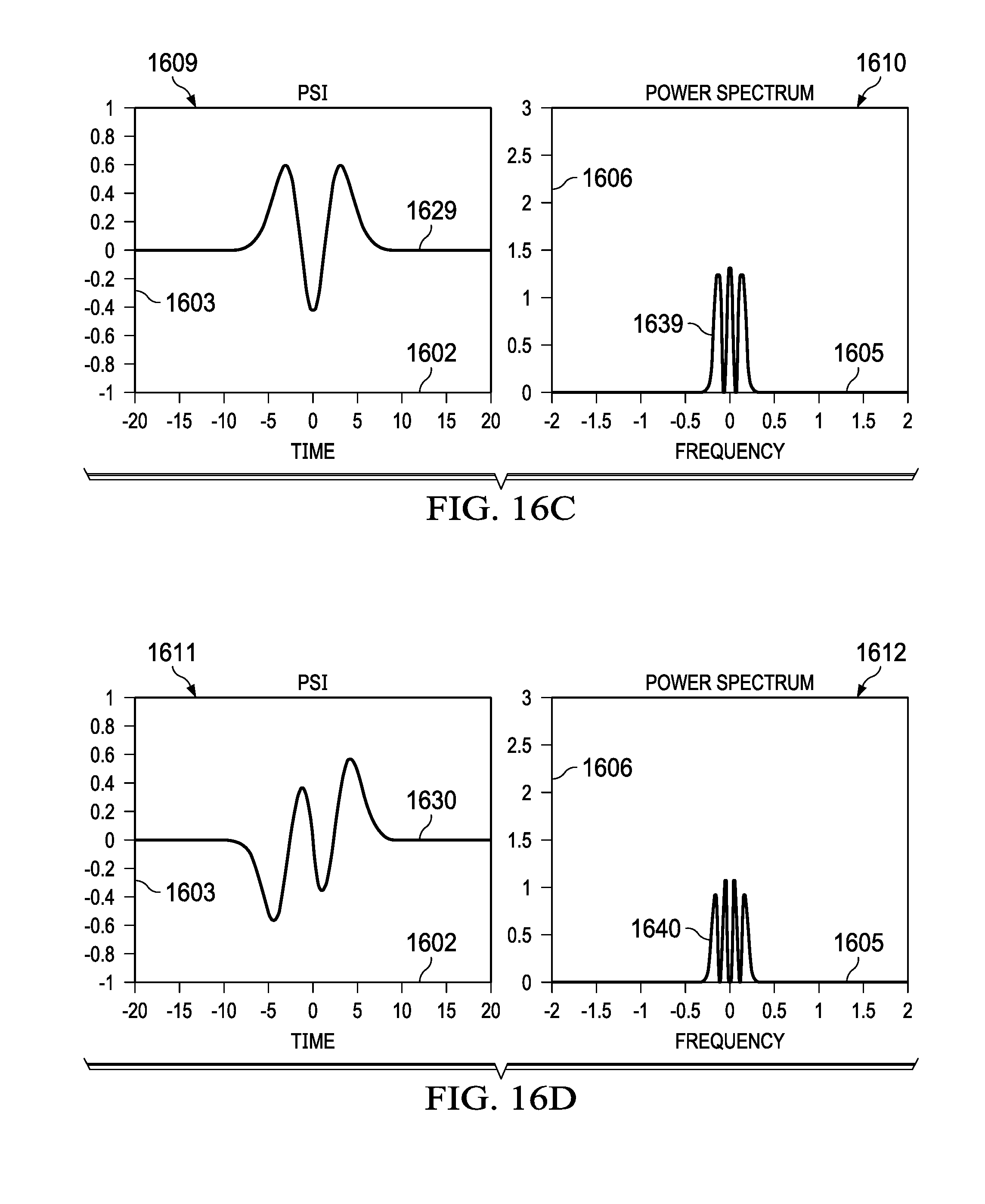
D00014

D00015

D00016

D00017
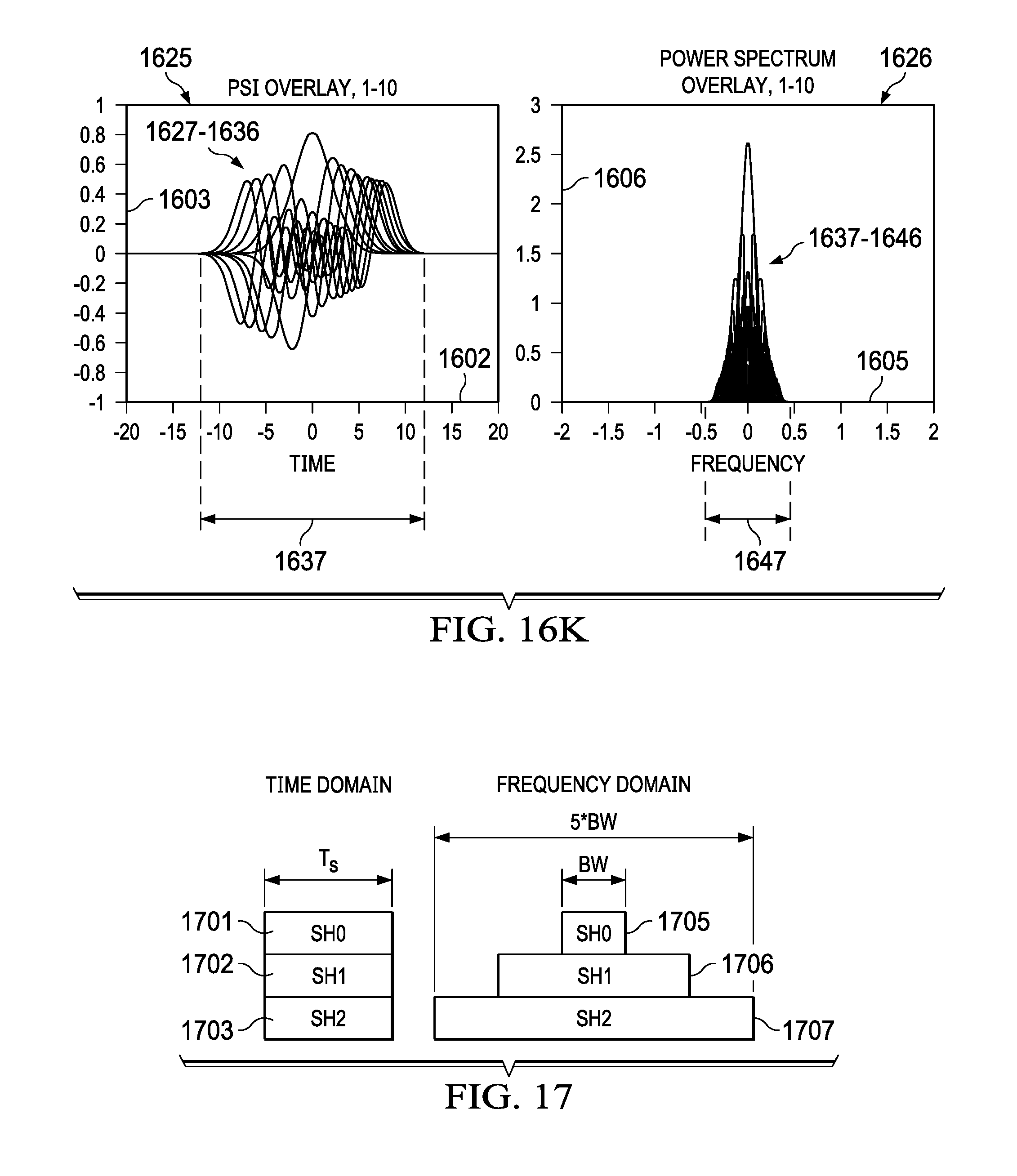
D00018

D00019
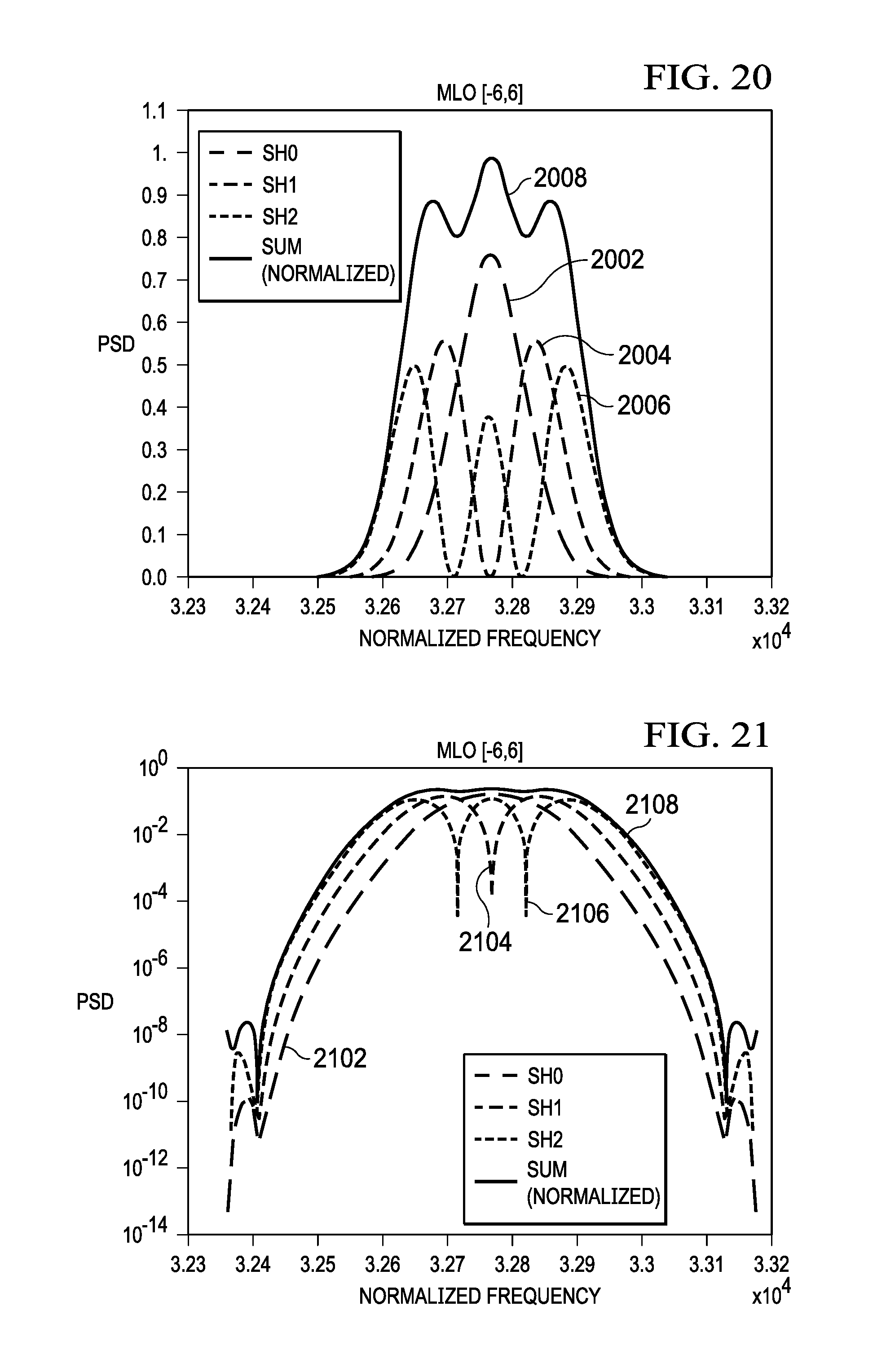
D00020

D00021
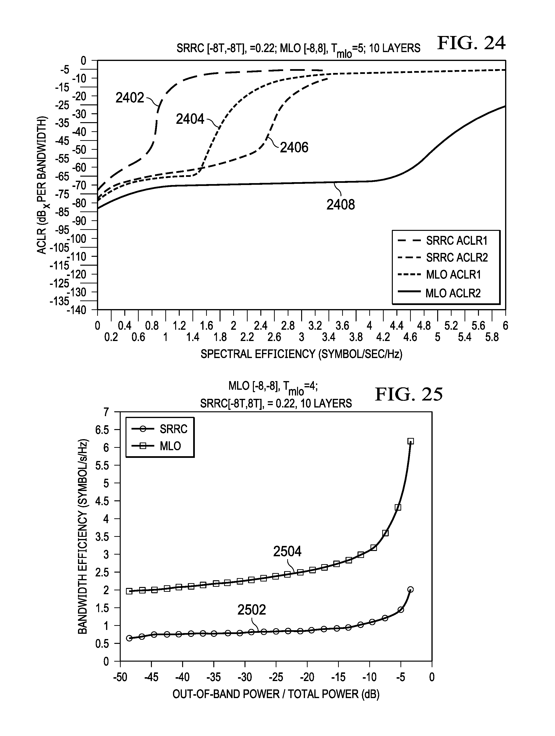
D00022

D00023
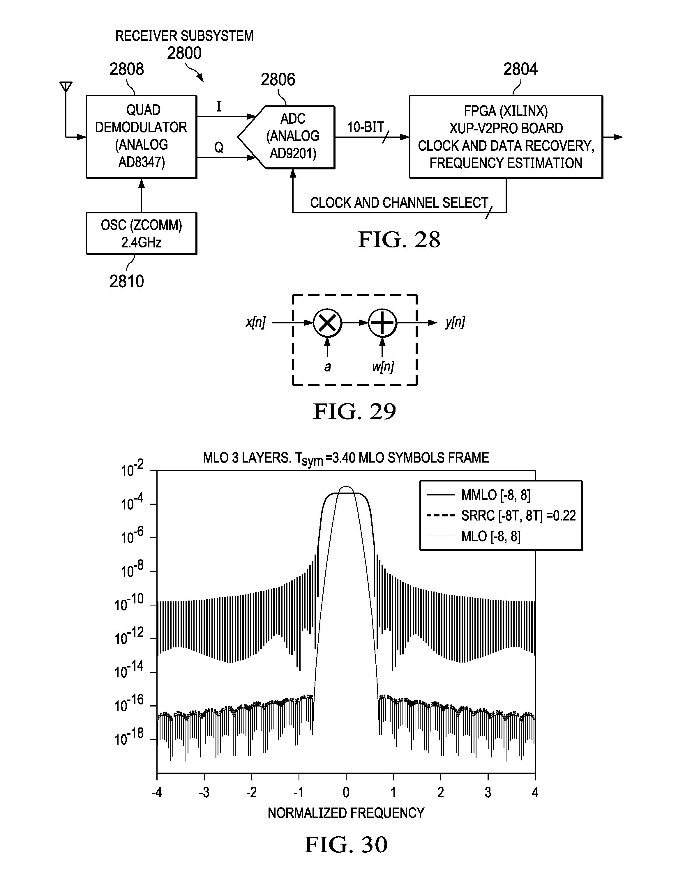
D00024

D00025
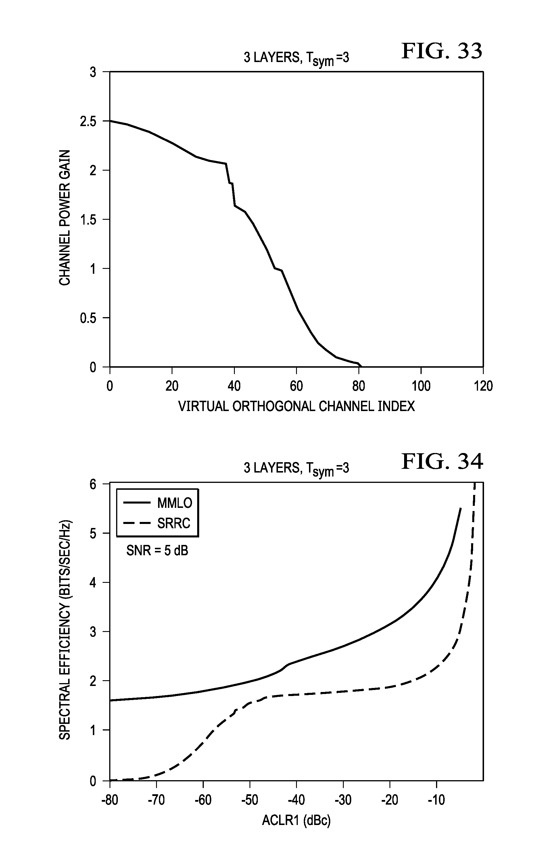
D00026

D00027

D00028
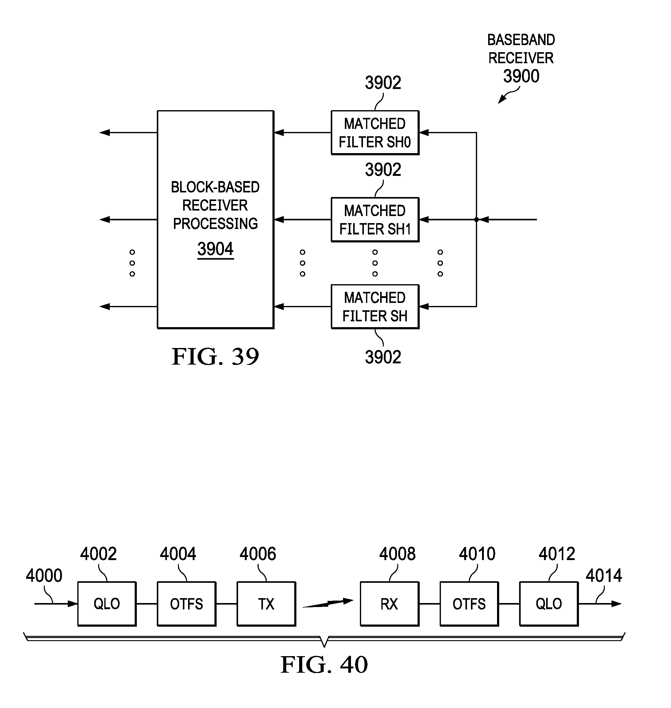
D00029

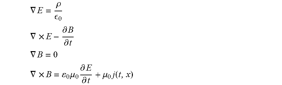
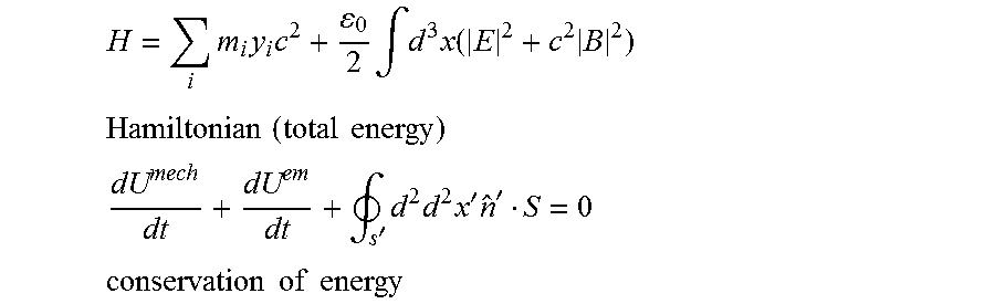


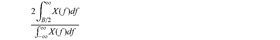


P00001

P00002

P00003

P00004

XML
uspto.report is an independent third-party trademark research tool that is not affiliated, endorsed, or sponsored by the United States Patent and Trademark Office (USPTO) or any other governmental organization. The information provided by uspto.report is based on publicly available data at the time of writing and is intended for informational purposes only.
While we strive to provide accurate and up-to-date information, we do not guarantee the accuracy, completeness, reliability, or suitability of the information displayed on this site. The use of this site is at your own risk. Any reliance you place on such information is therefore strictly at your own risk.
All official trademark data, including owner information, should be verified by visiting the official USPTO website at www.uspto.gov. This site is not intended to replace professional legal advice and should not be used as a substitute for consulting with a legal professional who is knowledgeable about trademark law.