A Dynamically Non-gaussian Anomaly Identification Method For Structural Monitoring Data
YI; Tinghua ; et al.
U.S. patent application number 16/090911 was filed with the patent office on 2019-04-25 for a dynamically non-gaussian anomaly identification method for structural monitoring data. The applicant listed for this patent is Dalian University of Technology. Invention is credited to Haibin HUANG, Hongnan LI, Tinghua YI.
| Application Number | 20190121838 16/090911 |
| Document ID | / |
| Family ID | 59184032 |
| Filed Date | 2019-04-25 |

| United States Patent Application | 20190121838 |
| Kind Code | A1 |
| YI; Tinghua ; et al. | April 25, 2019 |
A DYNAMICALLY NON-GAUSSIAN ANOMALY IDENTIFICATION METHOD FOR STRUCTURAL MONITORING DATA
Abstract
The present invention belongs to the technical field of health monitoring for civil structures, and a dynamically non-Gaussian anomaly identification method is proposed for structural monitoring data. First, define past and current observation vectors for the monitoring data and pre-whiten them; second, establish a statistical correlation model for the whitened past and current observation vectors to obtain dynamically whitened data; then, divide the dynamically whitened data into two parts, i.e., the system-related and system-unrelated parts, which are further modelled by the independent component analysis; finally, define two statistics and determine their corresponding control limits, respectively, it can be decided that there is anomaly in the monitoring data when each of the statistics exceeds its corresponding control limit. The non-Gaussian and dynamic characteristics of structural monitoring data are simultaneously taken into account, based on that the defined statistics can effectively identify anomalies in the data.
| Inventors: | YI; Tinghua; (Dalian City, Liaoning Province, CN) ; HUANG; Haibin; (Dalian City, Liaoning Province, CN) ; LI; Hongnan; (Dalian City, Liaoning Province, CN) | ||||||||||
| Applicant: |
|
||||||||||
|---|---|---|---|---|---|---|---|---|---|---|---|
| Family ID: | 59184032 | ||||||||||
| Appl. No.: | 16/090911 | ||||||||||
| Filed: | February 12, 2018 | ||||||||||
| PCT Filed: | February 12, 2018 | ||||||||||
| PCT NO: | PCT/CN2018/076577 | ||||||||||
| 371 Date: | October 3, 2018 |
| Current U.S. Class: | 1/1 |
| Current CPC Class: | G06K 9/6247 20130101; G06F 30/20 20200101; G06K 9/00 20130101; G06K 9/00523 20130101; G06K 9/624 20130101; G06K 9/6297 20130101; G06K 9/00536 20130101; G01M 5/0008 20130101; G06F 17/18 20130101 |
| International Class: | G06F 17/18 20060101 G06F017/18 |
Foreign Application Data
| Date | Code | Application Number |
|---|---|---|
| Feb 16, 2017 | CN | 201710084131.6 |
Claims
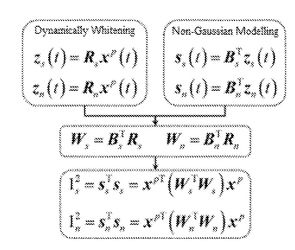
1. A dynamically non-Gaussian anomaly identification method for structural monitoring data, wherein, the specific steps of which are as follows: Step 1: Structural monitoring data preprocessing (1) Let x(t) .di-elect cons. .sup.m represent a sample at time t in the normal structural monitoring data, where m is the number of measurement variables; define the past observation vector x.sup.p(t)=[x.sup.T(t-1), x.sup.T(t-2), . . . , x.sup.T(t-.tau.)].sup.T (note: .tau. is the time-lag) and the current observation vector x.sup.c(t)=x(t); (2) Let J.sup.p and J.sup.c represent whitening matrices corresponding to x.sup.p(t) and x.sup.c(t), respectively, the whitened x.sup.p(t) and x.sup.c(t) can be obtained by {tilde over (x)}.sup.p(t)=J.sup.px.sup.p(t) and {tilde over (x)}.sup.c(t)=J.sup.cx.sup.c(t), respectively; Step 2: Dynamically whitening (3) Dynamically modeling of structural monitoring data is to establish a statistical correlation model between {tilde over (x)}.sup.p(t) and {tilde over (x)}.sup.c(t): {tilde over (S)}.sub.pc=E{{tilde over (x)}.sup.p{tilde over (x)}.sup.cT}=P.SIGMA.Q.sup.T where {tilde over (S)}.sub.pc represents the cross-covariance matrix of {tilde over (x)}.sup.p and {tilde over (x)}.sup.c; P .di-elect cons. .sup.m.tau..times.m.tau. and Q .di-elect cons. .sup.m.times.m represent matrices consisting all left and right singular vectors of singular value decomposition, respectively; .SIGMA. .di-elect cons. .sup.m.tau..times.m represents the singular value matrix, which contains in non-zero singular values; (4) Define the projection of {tilde over (x)}.sup.p(t) on P, termed as z(t), which can be calculated by the following equation: z(t)=P.sup.T{tilde over (x)}.sup.p(t)=P.sup.TJ.sup.px.sup.p(t)=Rx.sup.p(t) where R=P.sup.TJ.sup.p; (5) Since the covariance matrix of z(t) is an identity matrix: S.sub.zz=E{zz.sup.T}=P.sup.TE{{tilde over (x)}.sup.p{tilde over (x)}.sup.pT}P=I and the above modeling process takes into account the dynamic characteristics of structural monitoring data, R can be termed as dynamically whitening matrix and z(t) can be termed as dynamically whitened data; Step 3: Dynamically non-Gaussian modelling (6) Divide the dynamically whitened data z(t) into two parts using the following equations: z.sub.s(t)=R.sub.sx.sup.p(t) z.sub.n(t)=R.sub.nx.sup.p(t) where z.sub.s(t) and z.sub.n(t) represent the system-related and system-unrelated parts of z(t), respectively; R.sub.s and R.sub.n are consist of the first m rows and last m(l-1) rows of R, respectively; (7) Establish dynamically non-Gaussian models for z.sub.s(t) and z.sub.n(t) using independent component analysis: s.sub.s(t)=B.sub.s.sup.Tz.sub.s(t) s.sub.n(t)=B.sub.n.sup.Tz.sub.n(t) where s.sub.s(t) and s.sub.n(t) represent system-related and system-unrelated independent components, respectively; B.sub.s and B.sub.n can be solved by the fast independent component analysis algorithm; (8) Let W.sub.s=B.sub.s.sup.TR.sub.s and W.sub.n=B.sub.n.sup.TR.sub.n, there exist the following equations: s.sub.s(t)=W.sub.sx.sup.p(t) s.sub.n(t)=W.sub.nx.sup.p(t) where W.sub.s and W.sub.n represent de-mixing matrices corresponding to the system-related and system-unrelated parts, respectively; Step 4: Define statistics and determine control limits (9) Define two statistics corresponding to s.sub.s(t) and s.sub.n(t), respectively: I.sub.s.sup.2=s.sub.s.sup.Ts.sub.s=x.sup.pT(W.sub.s.sup.TW.sub.s)x.sup.p I.sub.n.sup.2=s.sub.n.sup.Ts.sub.n=x.sup.pT(W.sub.n.sup.TW.sub.n)x.sup.p (10) After calculating the statistics I.sub.s.sup.2 and I.sub.n.sup.2 for all normal structural monitoring data, estimate the probability density distribution of I.sub.s.sup.2 and I.sub.n.sup.2, respectively; determine the control limits I.sub.s,lim.sup.2 and I.sub.n,lim.sup.2 of the two statistics through the 99% confidence criterion; it can be decided that there exist anomalies in the newly acquired monitoring data, when each of the statistics exceeds its corresponding control limit.
Description
TECHNICAL FIELD
[0001] The present invention belongs to the technical field of health monitoring for civil structures, and a dynamically non-Gaussian anomaly identification method is proposed for structural monitoring data.
BACKGROUND
[0002] The service performance of civil structures will inevitably deteriorate due to the collective effects of long-term loadings, environmental corrosion and fatigue factors. Through in-depth analysis of structural monitoring data, the abnormal condition of structures can be discovered in time and an accurate safety early-warning can then be provided, which has important practical significance for ensuring the safe operation of civil structures. At present, the anomaly identification of structural monitoring data is mainly achieved through statistical methods, which can be generally divided into two categories: 1) the univariate control chart, such as the Shewhart control chart, the CUSUM control chart and so forth, which is used to establish separate control chart for the monitoring data at each measurement point to identify anomalies in the monitoring data; and 2) the multivariate statistical analysis, such as the principal component analysis, the independent component analysis and so forth, which employs the correlation between monitoring data at multiple measurement points to establish a statistical model, and then defines corresponding statistics to identify anomalies in the monitoring data.
[0003] Due to the deformation continuity of structures, there exists correlation between structural response data at the adjacent measurement points. In practical engineering applications, multivariate statistical analysis is more advantageous since this kind of correlation can be considered. However, due to various factors, such as the structural nonlinearity, the complexity of measurement noise and so forth, structural monitoring data often exhibits non-Gaussian properties; in addition, dynamic characteristics (i.e., autocorrelation) also exist in structural monitoring data. If non-Gaussian and dynamic characteristics can be considered simultaneously in the modeling process of structural monitoring data, the anomaly identification ability of the multivariate statistical analysis method can be improved, making it more practical in engineering applications.
SUMMARY
[0004] The present invention aims to propose a dynamically non-Gaussian modeling method for structural monitoring data, based on that two statistics are defined to identify anomalies in the data. The technical solution of the present invention is as follows: first, define past and current observation vectors for the monitoring data and pre-whiten them; second, establish a statistical correlation model for the whitened past and current observation vectors to obtain dynamically whitened data; then, divide the dynamically whitened data into two parts, i.e., the system-related and system-unrelated parts, which are further modelled by the independent component analysis; finally, define two statistics and determine their corresponding control limits, respectively, it can be decided that there is anomaly in the monitoring data when each of the statistics exceeds its corresponding control limit.
[0005] A dynamically non-Gaussian anomaly identification method for structural monitoring data, the specific steps of which are as follows:
[0006] Step 1: Structural monitoring data preprocessing
[0007] (1) Let x(t) .di-elect cons. .sup.m represent a sample at time t in the normal structural monitoring data, where m is the number of measurement variables; define the past observation vector x.sup.p(t)=[x.sup.T(t-1), x.sup.T(t-2), . . . , x.sup.T(t-.tau.)].sup.T (note: .tau. is the time-lag) and the current observation vector x.sup.c(t)=x(t);
[0008] (2) Let J.sup.p and J.sup.c represent whitening matrices corresponding to x.sup.p(t) and x.sup.c(t), respectively, the whitened x.sup.p(t) and x.sup.c(t) can be obtained by {tilde over (x)}.sup.p(t)=J.sup.px.sup.p(t) and {tilde over (x)}.sup.c(t)=J.sup.cx.sup.c(t), respectively;
[0009] Step 2: Dynamically whitening
[0010] (3) Dynamically modeling of structural monitoring data is to establish a statistical correlation model between {tilde over (x)}.sup.p(t) and {tilde over (x)}.sup.c(t):
{tilde over (S)}.sub.pc=E{{tilde over (x)}.sup.p{tilde over (x)}.sup.cT}=P.SIGMA.Q.sup.T
where {tilde over (S)}.sub.pc represents the cross-covariance matrix of {tilde over (x)}.sup.p and {tilde over (x)}.sup.c; P .di-elect cons. .sup.m.tau..times.m.tau. and Q .di-elect cons. .sup.m.times.m represent matrices consisting all left and right singular vectors of singular value decomposition, respectively; .SIGMA. .di-elect cons. .sup.m.tau..times.m represents the singular value matrix, which contains m non-zero singular values;
[0011] (4) Define the projection of {tilde over (x)}.sup.p(t) on P, termed as z(t), which can be calculated by the following equation:
z(t)=P.sup.T{tilde over (x)}.sup.p(t)=P.sup.TJ.sup.px.sup.p(t)=Rx.sup.p(t)
where R=P.sup.TJ.sup.p;
[0012] (5) Since the covariance matrix of z(t) is an identity matrix:
S.sub.zz=E{zz.sup.T}=P.sup.TE{{tilde over (x)}.sup.p{tilde over (x)}.sup.pT}P=I
and the above modeling process takes into account the dynamic characteristics of structural monitoring data, R can be termed as dynamically whitening matrix and z(t) can be termed as dynamically whitened data;
[0013] Step 3: Dynamically non-Gaussian modelling
[0014] (6) Divide the dynamically whitened data z(t) into two parts using the following equations:
z.sub.s(t)=R.sub.sx.sup.p(t)
z.sub.n(t)=R.sub.nx.sup.p(t)
where z.sub.s(t) and z.sub.n(t) represent the system-related and system-unrelated parts of z(t), respectively; R.sub.s and R.sub.n are consist of the first m rows and last m(l-1) rows of R, respectively;
[0015] (7) Establish dynamically non-Gaussian models for z.sub.s(t) and z.sub.n(t) using independent component analysis:
s.sub.s(t)=B.sub.s.sup.Tz.sub.s(t)
s.sub.n(t)=B.sub.n.sup.Tz.sub.n(t)
where s.sub.s(t) and s.sub.n(t) represent system-related and system-unrelated independent components, respectively; B.sub.s and B.sub.n can be solved by the fast independent component analysis algorithm;
[0016] (8) Let W.sub.s=B.sub.s.sup.TR.sub.s and W.sub.n=B.sub.n.sup.TR.sub.n, there exist the following equations:
s.sub.s(t)=W.sub.sx.sup.p(t)
s.sub.n(t)=W.sub.nx.sup.p(t)
where W.sub.s and W.sub.n represent de-mixing matrices corresponding to the system-related and system-unrelated parts, respectively;
[0017] Step 4: Define statistics and determine control limits
[0018] (9) Define two statistics corresponding to s.sub.s(t) and s.sub.n(t), respectively:
I.sub.s.sup.2=s.sub.s.sup.Ts.sub.s=x.sup.pT(W.sub.s.sup.TW.sub.s)x.sup.p
I.sub.n.sup.2=s.sub.n.sup.Ts.sub.n=x.sup.pT(W.sub.n.sup.TW.sub.n)x.sup.p
[0019] (10) After calculating the statistics (i.e., I.sub.s.sup.2 and I.sub.n.sup.2) for all normal structural monitoring data, estimate the probability density distribution of I.sub.s.sup.2 and I.sub.n.sup.2, respectively; determine the control limits (i.e., I.sub.s,lim.sup.2 and I.sub.n,lim.sup.2) of the two statistics through the 99% confidence criterion; it can be decided that there exist anomalies in the newly acquired monitoring data, when each of the statistics exceeds its corresponding control limit.
[0020] The present invention has the beneficial effect that: the non-Gaussian and dynamic characteristics of structural monitoring data are simultaneously taken into account in the process of statistical modeling, based on that the defined statistics can effectively identify anomalies in the data.
DETAILED DESCRIPTION
[0021] The following details is used to further describe the specific implementation process of the present invention.
[0022] Take a two-span highway bridge model, with a length of 5.4864 m and a width of 1.8288 m, as an example. A finite element model is built to simulate structural responses, and the responses at 12 finite element nodes are acquired as monitoring data. There are two datasets generated: the training dataset and the testing dataset; the training dataset consists of normal monitoring data, and part of the testing dataset is used to simulate abnormal monitoring data; both datasets last for 80 s and the sampling frequency is 256 Hz. The basic idea of the present invention is shown in the following schematic:
[0023] (1) Construct the past observation vector x.sup.p(t) and the current observation vector x.sup.c(t) for each data point in the training dataset then pre-whiten all past and current observation vectors (i.e., x.sup.p(t) and x.sup.c(t)) to obtain the whitening matrices (i.e., J.sup.p and J.sup.c) and the whitened past and current observation vectors (i.e., {tilde over (x)}.sup.p(t) and {tilde over (x)}.sup.c(t)).
[0024] (2) Establish a statistical correlation model for {tilde over (x)}.sup.p(t) and {tilde over (x)}.sub.c(t) to obtain the dynamically whitening matrix R; the first 12 rows of R are used to construct R.sub.s and the others are used to construct R.sub.n; calculate z.sub.s(t)=R.sub.sx.sup.p(t) and z.sub.n(t)=R.sub.nx.sup.p(t).
[0025] (3) Establish independent component analysis models for z.sub.s(t) and z.sub.n(t) to obtain matrices B.sub.s and B.sub.n; correspondingly, the de-mixing matrices can be obtained through W.sub.s=B.sub.s.sup.TR.sub.s and W.sub.n=B.sub.n.sup.TR.sub.n; calculate statistics I.sub.s.sup.2 and I.sub.n.sup.2, then determine their corresponding control limits I.sub.s,lim.sup.2 and I.sub.n,lim.sup.2; it can be decided that there exist anomalies in the data when each of the statistics exceeds its corresponding control limit.
[0026] (4) Simulate abnormal monitoring data in the testing dataset, that is, the monitoring data of sensor 2 gains anomaly during time 40.about.80 s; identify anomalies in the monitoring data using the two proposed statistics I.sub.s.sup.2 and I.sub.n.sup.2, results show that both I.sub.s.sup.2 and I.sub.n.sup.2 can successfully identify anomalies in the monitoring data.
* * * * *
P00001
P00002
XML
uspto.report is an independent third-party trademark research tool that is not affiliated, endorsed, or sponsored by the United States Patent and Trademark Office (USPTO) or any other governmental organization. The information provided by uspto.report is based on publicly available data at the time of writing and is intended for informational purposes only.
While we strive to provide accurate and up-to-date information, we do not guarantee the accuracy, completeness, reliability, or suitability of the information displayed on this site. The use of this site is at your own risk. Any reliance you place on such information is therefore strictly at your own risk.
All official trademark data, including owner information, should be verified by visiting the official USPTO website at www.uspto.gov. This site is not intended to replace professional legal advice and should not be used as a substitute for consulting with a legal professional who is knowledgeable about trademark law.