Receiver-side Processing Of Orthogonal Time Frequency Space Modulated Signals
Hadani; Ronny ; et al.
U.S. patent application number 16/084791 was filed with the patent office on 2019-03-14 for receiver-side processing of orthogonal time frequency space modulated signals. The applicant listed for this patent is COHERE TECHNOLOGIES. Invention is credited to Clayton Ambrose, Anthony Ekpenyong, Ronny Hadani, Shachar Kons, Shlomo Selim Rakib.
| Application Number | 20190081836 16/084791 |
| Document ID | / |
| Family ID | 59899748 |
| Filed Date | 2019-03-14 |

View All Diagrams
| United States Patent Application | 20190081836 |
| Kind Code | A1 |
| Hadani; Ronny ; et al. | March 14, 2019 |
RECEIVER-SIDE PROCESSING OF ORTHOGONAL TIME FREQUENCY SPACE MODULATED SIGNALS
Abstract
Wireless communication techniques for transmitting and receiving reference signals is described. The reference signals may include pilot signals that are transmitted using transmission resources that are separate from data transmission resources. Pilot signals are continuously transmitted from a base station to user equipment being served. Pilot signals are generated from delay-Doppler domain signals that are processed to obtain time-frequency signals that occupy a two-dimensional lattice in the time frequency domain that is non-overlapping with a lattice corresponding to data signal transmissions.
| Inventors: | Hadani; Ronny; (Santa Clara, CA) ; Rakib; Shlomo Selim; (Santa Clara, CA) ; Ekpenyong; Anthony; (Santa Clara, CA) ; Ambrose; Clayton; (Santa Clara, CA) ; Kons; Shachar; (Santa Clara, CA) | ||||||||||
| Applicant: |
|
||||||||||
|---|---|---|---|---|---|---|---|---|---|---|---|
| Family ID: | 59899748 | ||||||||||
| Appl. No.: | 16/084791 | ||||||||||
| Filed: | March 23, 2017 | ||||||||||
| PCT Filed: | March 23, 2017 | ||||||||||
| PCT NO: | PCT/US17/23892 | ||||||||||
| 371 Date: | September 13, 2018 |
Related U.S. Patent Documents
| Application Number | Filing Date | Patent Number | ||
|---|---|---|---|---|
| 62312367 | Mar 23, 2016 | |||
| Current U.S. Class: | 1/1 |
| Current CPC Class: | H04L 1/0045 20130101; H04L 27/2697 20130101; H04L 5/0007 20130101; H04L 27/2647 20130101; H04L 27/2639 20130101; H04B 7/0413 20130101; H04L 27/2613 20130101; H04L 5/00 20130101; H04L 27/2634 20130101; H04L 27/265 20130101; H04L 5/0048 20130101; H04L 5/0023 20130101 |
| International Class: | H04L 27/26 20060101 H04L027/26; H04L 5/00 20060101 H04L005/00 |
Claims
1. A wireless communication method, implemented by a wireless communication receiver, comprising: processing a wireless signal comprising information bits modulated using an orthogonal time frequency and space (OTFS) modulation scheme to generate time-frequency domain digital samples; performing linear equalization of the time-frequency domain digital samples resulting in an equalized signal; and inputting the equalized signal to a feedback filter operated in a delay-time domain to produce a decision feedback equalizer (DFE) output signal; extracting symbol estimates from the DFE output signal; and recovering the information bits from the symbol estimates.
2. The method of claim 1, wherein the extracting symbol estimates is performed in a delay-Doppler domain.
3. The method of claim 1, wherein the processing the wireless signal includes applying a two-dimensional transform to generate the time-frequency domain digital samples.
4. The method of claim 3, wherein the two-dimensional transform comprises a discrete Symplectic Fourier transform.
5. The method of claim 3, wherein the applying the two-dimensional transform includes applying a two-dimensional windowing function over a grid in the time-frequency domain.
6-9. (canceled)
10. The method of claim 1, wherein the performing the linear equalization includes performing Wiener filtering of the time-frequency domain digital samples.
11. (canceled)
12. The method of claim 1, wherein the producing the DFE output signal includes performing a single input multi-output (SIMO) decision feedback equalization (DFE) to produce the DFE output signal.
13-14. (canceled)
15. The method of claim 13, wherein the DFE is performed by operating a set of M parallel noise-predictive DFE feedback filters in the delay-time domain, where M is an integer.
16. The method of claim 15, further including: computing an output of the equalizer by: transforming, for a given OTFS symbol, the output of the equalizer to a delay-time domain representation; computing an estimate of a delay-domain error covariance matrix; computing a truncated error covariance matrix; obtaining filter coefficients of a feedforward filter; and calculating the output of the equalizer using the filter coefficients.
17. A wireless communication receiver apparatus, comprising: a radio frequency (RF) front end; a memory storing instructions; a processor that reads the instructions from memory to receive a wireless signal from the RF front end and recover information bits from the wireless signal, the instructions comprising: instructions for processing a wireless signal comprising information bits modulated using an orthogonal time frequency and space (OTFS) modulation scheme to generate time-frequency domain digital samples; instructions for performing linear equalization of the time-frequency domain digital samples resulting in an equalized signal; and instructions for inputting the equalized signal to a feedback filter operated in a delay-time domain to produce a decision feedback equalizer (DFE) output signal; instructions for extracting symbol estimates from the DFE output signal; and instructions for recovering the information bits from the symbol estimates.
18. The apparatus of claim 17, wherein the instructions for extracting symbol estimates include instructions for extracting symbol estimates in a delay-Doppler domain.
19. The apparatus of claim 17, wherein the instructions for processing the wireless signal include instructions for applying a two-dimensional transform to generate the time-frequency domain digital samples.
20. The apparatus of claim 19, wherein the two-dimensional transform comprises a discrete Symplectic Fourier transform.
21. The apparatus of claim 19, wherein the instructions for applying the two-dimensional transform include instructions for applying a two-dimensional windowing function over a grid in the time-frequency domain.
22-25. (canceled)
26. The apparatus of claim 17, wherein the instructions for performing the linear equalization include instructions for performing Wiener filtering of the time-frequency domain digital samples.
27. (canceled)
28. The apparatus of claim 17, wherein the instructions for producing the DFE output signal include instructions for performing a single input multi-output (SIMO) decision feedback equalization (DFE) to produce the DFE output signal.
29. The apparatus of claim 28, wherein the SIMO-DFE is performed by operating a set of M parallel noise-predictive DFE feedback filters in the delay-time domain, where M is an integer.
30. The apparatus of claim 29, wherein the instructions further include: instructions for computing an output of the equalizer by: instructions for transforming, for a given OTFS symbol, the output of the equalizer to a delay-time domain representation; instructions for computing an estimate of a delay-domain error covariance matrix; instructions for computing a truncated error covariance matrix; instructions for obtaining filter coefficients of a feedforward filter; and instructions for calculating the output of the equalizer using the filter coefficients.
31. The apparatus of claim 17, wherein the instructions for producing the DFE output signal include instructions for performing a multi-input multi-output (MIMO) decision feedback equalization (DFE) to produce the DFE output signal.
32. (canceled)
33. The method of claim 1, wherein the wireless signal comprises one or more streams and wherein each stream comprises a first portion that includes a pilot signal, and a second portion in which data being transmitted to multiple user equipment is arranged in increasing level of modulation constellation density along a delay dimension.
34. (canceled)
Description
CROSS-REFERENCE TO RELATED APPLICATIONS
[0001] This patent document claims priority to U.S. Provisional Application Ser. No. 62/257,171, entitled "RECEIVER-SIDE PROCESSING OF ORTHOGONAL TIME FREQUENCY SPACE MODULATED SIGNALS" filed on Mar. 23, 2016. The entire content of the aforementioned patent application is incorporated by reference herein.
TECHNICAL FIELD
[0002] The present document relates to wireless communication, and more particularly, to receiver-side processing of orthogonal time frequency space modulated signals.
BACKGROUND
[0003] Due to an explosive growth in the number of wireless user devices and the amount of wireless data that these devices can generate or consume, current wireless communication networks are fast running out of bandwidth to accommodate such a high growth in data traffic and provide high quality of service to users.
[0004] Various efforts are underway in the telecommunication industry to come up with next generation of wireless technologies that can keep up with the demand on performance of wireless devices and networks.
SUMMARY
[0005] This document discloses receiver-side techniques for receiving orthogonal time frequency and space (OTFS) modulated signals, and extracting information bits therefrom.
[0006] In one example aspect, a wireless communication method, implemented by a wireless communications receiver is disclosed. The method includes processing a wireless signal comprising information bits modulated using an orthogonal time frequency and space (OTFS) modulation scheme to generate time-frequency domain digital samples, performing linear equalization of the time-frequency domain digital samples resulting in an equalized signal, inputting the equalized signal to a feedback filter operated in a delay-time domain to produce a decision feedback equalizer (DFE) output signal, extracting symbol estimates from the DFE output signal, and recovering the information bits from the symbol estimates.
[0007] In another example aspect, an apparatus for wireless communication is disclosed. The apparatus includes a module for processing a wireless signal received at one or more antennas of the apparatus. A module may perform linear equalization in the time-frequency domain. A module may perform DFE operation in the delay-time domain. A module may perform symbol estimation in the delay-Doppler domain.
[0008] These, and other, features are described in this document.
DESCRIPTION OF THE DRAWINGS
[0009] Drawings described herein are used to provide a further understanding and constitute a part of this application. Example embodiments and illustrations thereof are used to explain the technology rather than limiting its scope.
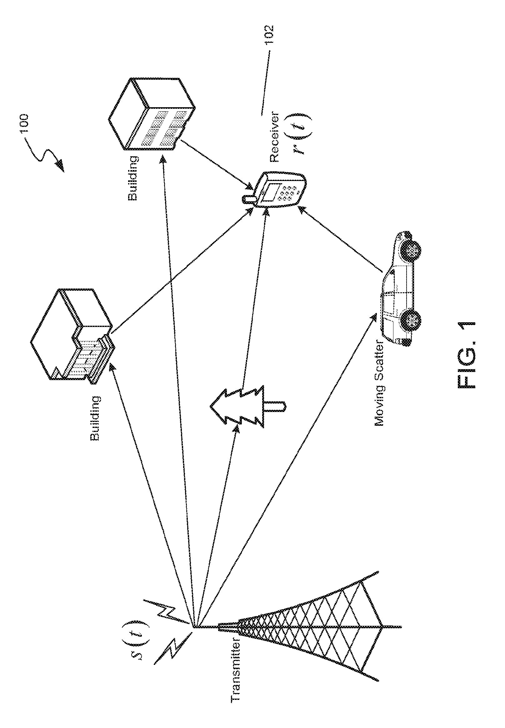
[0010] FIG. 1 shows an example communication network.
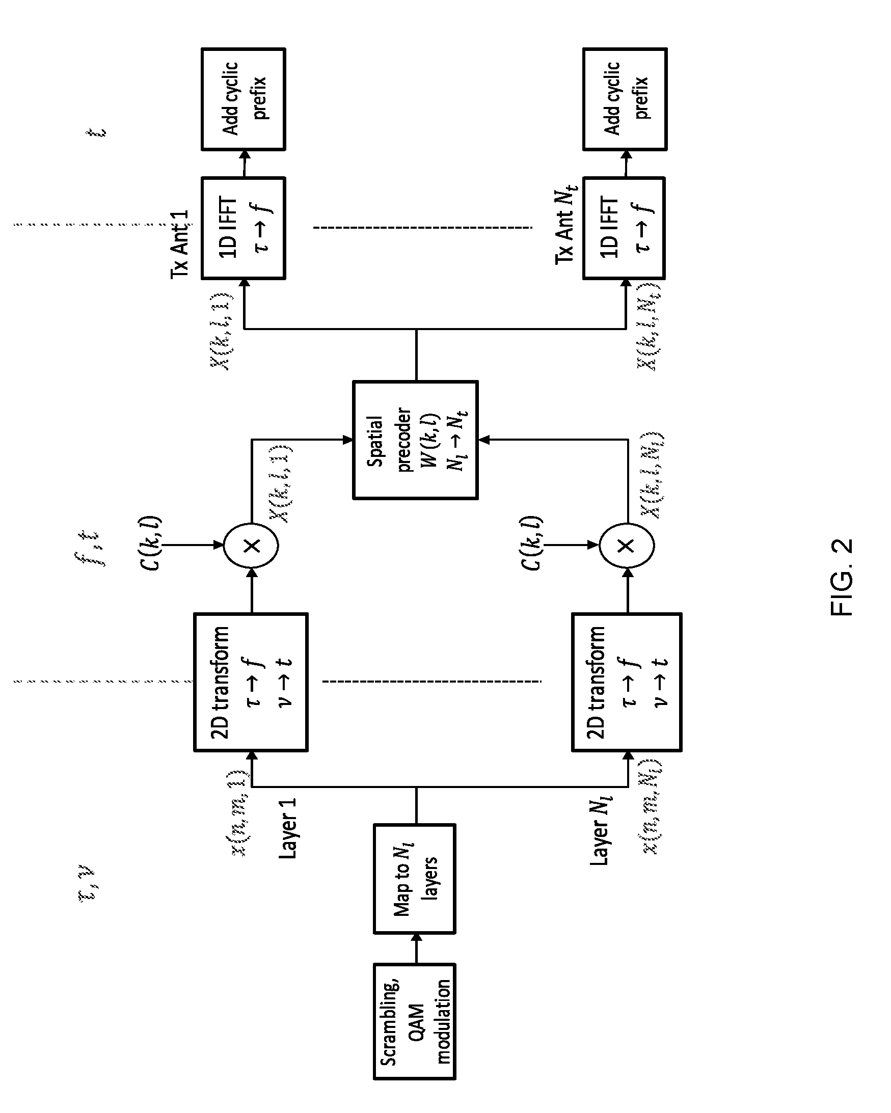
[0011] FIG. 2 is a block diagram showing an example of an OTFS transmitter.
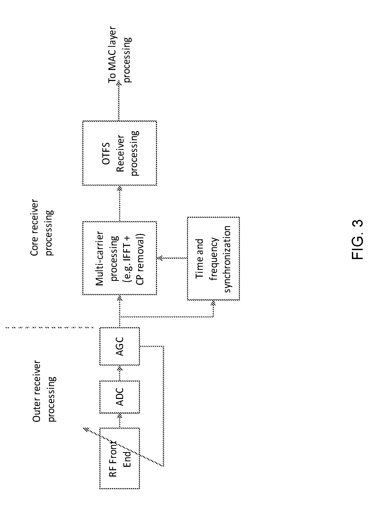
[0012] FIG. 3 is a block diagram showing an example of an OTFS receiver.
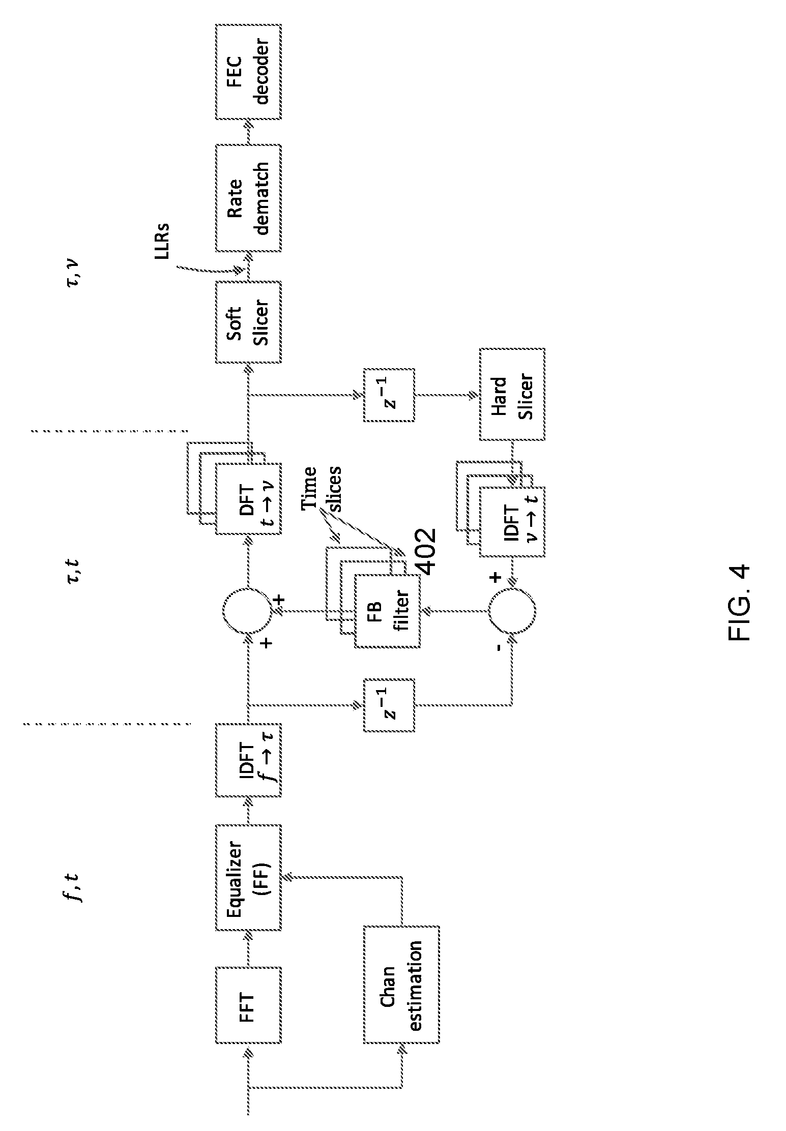
[0013] FIG. 4 is a block diagram showing an example of a single input multiple output (SIMO) DFE receiver.
[0014] FIG. 5 is a graph showing an example of multiplexing a pilot region and a data region in the delay-Doppler domain.
[0015] FIG. 6 is a block diagram showing an example of a MIMO DFE with ordered/unordered inter-stream interference cancellation (SIC).
[0016] FIG. 7 is a block diagram showing an example of a MIMO maximum likelihood (ML) DFE receiver which uses a hard slicer.
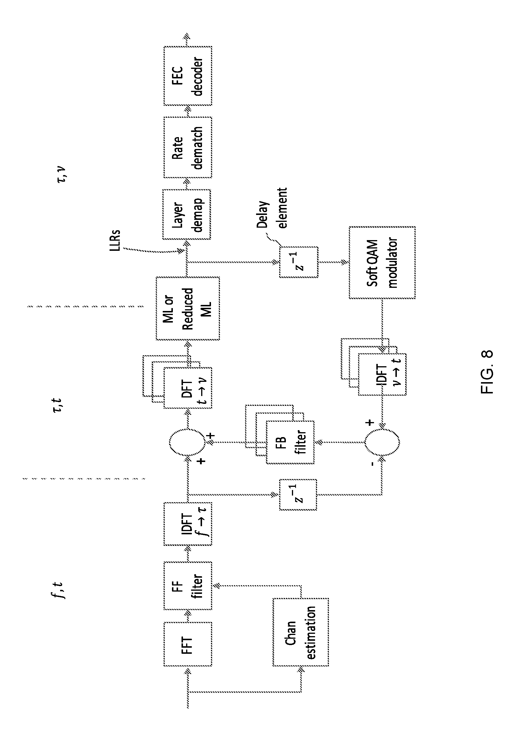
[0017] FIG. 8 is a block diagram showing an example of a MIMO ML-DFE receiver that uses soft-QAM modulation.
[0018] FIG. 9 shows a flowchart of an example wireless communication transmission method.
[0019] FIG. 10 shows a block diagram of an example of a wireless transmission apparatus.
[0020] FIG. 11 shows an example of a wireless transceiver apparatus.
[0021] FIG. 12 shows an example of a transmission frame.
DETAILED DESCRIPTION
[0022] To make the purposes, technical solutions and advantages of this disclosure more apparent, various embodiments are described in detail below with reference to the drawings. Unless otherwise noted, embodiments and features in embodiments of the present document may be combined with each other.
[0023] The present-day wireless technologies are expected to fall short in meeting the rising demand in wireless communications. Many industry organizations have started the efforts to standardize next generation of wireless signal interoperability standards. The 5th Generation (5G) effort by the 3rd Generation Partnership Project (3GPP) is one such example and is used throughout the document for the sake of explanation. The disclosed technique could be, however, used in other wireless networks and systems.
[0024] Section headings are used in the present document to improve readability of the description and do not in any way limit the discussion to the respective sections only.
[0025] FIG. 1 shows an example communication network 100 in which the disclosed technologies can be implemented. The network 100 may include a base station transmitter that transmits wireless signals s(t) (downlink signals) to one or more receivers 102, the received signal being denoted as r(t), which may be located in a variety of locations, including inside or outside a building and in a moving vehicle. The receivers may transmit uplink transmissions to the base station, typically located near the wireless transmitter. The technology described herein may be implemented at a receiver 102.
[0026] Because OTFS modulated signals are not modulated along a time-frequency grid but along a delay-Doppler grid, traditional signal reception techniques such as those used for receiving orthogonal frequency division multiplexing (OFDM) signals, for example, as used in Long Term Evolution (LTE) systems, cannot provide adequate performance to receive and process OTFS signals to extract or recover information bits modulated on the OTFS signals.
[0027] The presently disclosed techniques can overcome these problems, and others.
1. Introduction
[0028] Signal transmission over a wireless fading channel undergoes time and frequency selective fading which must be compensated for reliable end-to-end communication. Contemporary multi-carrier modulation techniques such as Orthogonal Frequency Division Multiplexing (OFDM) and Single Carrier Frequency Division Multiplexing (SC-FDM) exploit the degrees of freedom offered by the channel's frequency selectivity, which is characterized by the delay spread. However, the time-selective nature of the channel, as characterized by the Doppler spread, is not natively handled by these modulation techniques. Orthogonal Time Frequency and Space is a generalized two-dimensional multi-carrier modulation that fully exploits the degrees of freedom offered by the delay and Doppler dimensions of a wireless channel.
[0029] 1.1 Notation
[0030] The following mathematical notation is adopted in this patent document.
[0031] Boldface font are used to describe vectors and matrices. In most cases lower-case and upper-case letters denote vectors and matrices respectively. In some cases, such as for differentiating time and frequency vectors, upper-case letters may also be used for vectors in the frequency domain.
[0032] The superscripts (.).sup.T, (.)*, (.).sup.H denote, respectively, transpose, conjugate and conjugate transpose operators while denotes the Kronecker product.
[0033] The element in row i and column j of matrix A is denoted as A.sub.ij or A(i,j).
[0034] The matrix F.sub.N denotes a normalized N.times.N DFT matrix where F.sub.N(i,j)=(1/ {square root over (N)})e.sup.-j2.pi.ij/N.
[0035] I.sub.L denotes an L.times.L identity matrix, while O.sub.L.times.L denotes an L.times.L zero matrix.
[0036] .sup.M denotes the M-dimensional vector space over the field of complex numbers, and x.di-elect cons..sup.M represents an M-dimensional column vector.
[0037] N.sub.t,N.sub.r are, respectively, the number of transmit and receive antennas.
[0038] N.sub.l is the number of spatial layers or streams.
[0039] N,M are the dimensions of the lattice corresponding to the Delay and Doppler axes respectively.
[0040] X(k,l) represents a signal at the (k,l) point on the time-frequency grid, where k is the frequency index and l is the time index.
2. Signal Model
[0041] A multi-antenna communication system may include devices transmitting over a wireless fading channel with N.sub.t transmit antennas and N.sub.r receive antennas. FIG. 2 depicts an example of an OTFS transmitter. The information bits to be communicated from the transmitter may be encoded by a Forward Error Correction (FEC) block, rate matched to the number of bits the channel allocation can support, scrambled and modulated onto a discrete constellation denoted as .OMEGA.. The information bits may include user data that is locally generated or received from other equipment via a data input connection (not shown in the figure). For clarity, a Quadrature Amplitude Modulation (QAM) constellation example is discussed, but it is also possible to use some other digital constellation such as Phase Shift Keying.
[0042] The QAM symbols are mapped onto one or more spatial layers (or streams) according to the determined channel rank. For example, in downlink cellular transmission from a base station to a User Equipment (UE), the channel rank may be computed by the UE and fed back as channel state information (CSI) to the base station. Alternatively, in a Time Division Duplex (TDD) system, the base station derives the channel rank by exploiting uplink-downlink channel reciprocity.
[0043] For OTFS transmission, the information symbols for layer p can be viewed as functions defined on a two-dimensional Delay-Doppler plane, x(.tau.,v,p), p=0, . . . , N.sub.l-1. The two-dimensional Delay-Doppler channel model equation is characterized by a 2D cyclic convolution
.gamma. ( .tau. , v ) = h ( .tau. , v ) * 2 D x ( .tau. , v ) ( 1 ) ##EQU00001##
[0044] where the MIMO channel h(.tau.,v) is of dimension N.sub.r.times.N.sub.l and has finite support along the Delay and Doppler axes, and y(.tau.,v).di-elect cons..sup.N.sup.r is the received noiseless signal. The transmitted vector x(.tau.,v).di-elect cons..sup.N.sup.l is assumed to be zero mean and unity variance. Practically, the QAM symbols are mapped onto a lattice by sampling at N points on the r axis and M points on the v axis, i.e. x(n,m,p), where n=0, . . . , N-1 and m=0, . . . , M-1. For simplicity we will omit the layer indexing except where necessary.
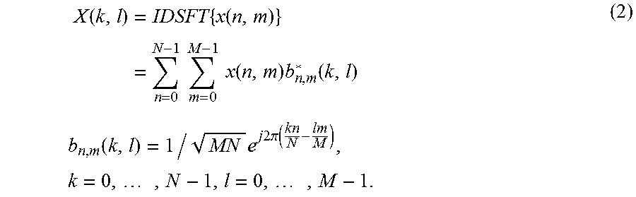
[0045] For each spatial layer, the information symbol matrix is transformed to the time-frequency domain by a two-dimensional transform. One such transform is the inverse Discrete Symplectic Fourier transform (IDSFT). The convention adopted in the present document about Symplectic Fourier transforms follows the 1-dimensional analogue. (1) (Continuous-time) Fourier transform (FT)<->Symplectic Fourier transform (SFT). (2) Discrete-time Fourier transform (DTFT)<->Discrete time-frequency Symplectic Fourier transform (DTFSFT). (3) Discrete Fourier transform (DFT)<->Discrete Symplectic Fourier transform (DSFT). The IDSFT converts the effect of the channel on the transmitted signal from a two-dimensional cyclic convolution in the Delay-Doppler domain to a multiplicative operation in the time-frequency domain. The IDSFT operation is given by the expression:
X ( k , l ) = IDSFT { x ( n , m ) } = n = 0 N - 1 m = 0 M - 1 x ( n , m ) b n , m * ( k , l ) b n , m ( k , l ) = 1 / MN e j 2 .pi. ( kn N - lm M ) , k = 0 , , N - 1 , l = 0 , , M - 1. ( 2 ) ##EQU00002##
[0046] It can be seen from the above that the IDSFT operation produces a 2D signal that is periodic in N and M.
[0047] Next, a windowing function, C(k,l), may be applied over the time-frequency grid. This windowing function serves multiple purposes. A first purpose is to randomize the time-frequency symbols. A second purpose is to apply a pseudo-random signature that distinguishes OTFS transmissions in a multiple access system. For example, C(k,l) may represent a signature sequence with low cross-correlation property to facilitate detection in a multi-point-to-point system such as the downlink of a wireless cellular network.
[0048] The spatial layers for each time-frequency grid point may be re-arranged into a vector at the input of the spatial precoder. The input to the spatial precoder for the (k,l) grid point is X.sub.kl=[X.sub.k,l(0), . . . , X.sub.k,l(N.sub.l-1)].sup.T. The spatial precoder W(k,l).di-elect cons..sup.N.sup.t.sup..times.N.sup.l transforms the N.sub.l layers to N.sub.t streams matching the number of transmit antennas. Subsequently, multi-carrier post-processing is applied, yielding the transmit waveform in the time domain. FIG. 2 shows an exemplary scheme, wherein a 1D IFFT is sequentially applied across the M OTFS time symbols. A cyclic prefix is added before the baseband signal is sent to a digital-to-analog converter and up-converted for transmission at the carrier frequency. In a different method a filter-bank may be applied rather than the IFFT+cyclic prefix method shown in FIG. 2.
[0049] FIG. 3 depicts an example of an OTFS receiver. From left to the right of the figure, he incoming RF signal is processed through an RF front end, which may include, but is not limited to, down-conversion to baseband frequency and other required processing such as low pass filtering, automatic frequency correction, IQ imbalance correction, and so on. The automatic gain control (AGC) loop and analog-to-digital conversion (ADC) blocks further process the baseband signal for input to the inner receiver sub-system. The time-and frequency synchronization system corrects for differences in timing between the transmitter and receiver sub-systems before multi-carrier processing. Herein, the multi-carrier processing may consist of cyclic prefix removal and FFT processing to convert the receive waveform to the time-frequency domain. In a different method, a filter-bank may be applied for multi-carrier processing.
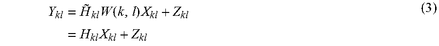
[0050] The received signal at the (k,l) time-frequency grid point is
Y kl = H ~ kl W ( k , l ) X kl + Z kl = H kl X kl + Z kl ( 3 ) ##EQU00003##
[0051] Where {tilde over (H)}.sub.kl.di-elect cons..sup.N.sup.r.sup..times.N.sup.t is the MIMO channel with each entry modeled as a complex Gaussian random variable [{tilde over (H)}.sub.kl].sub.ij.about.(0,1), and H.sub.kl.di-elect cons..sup.N.sup.r.sup..times.N.sup.l is the equivalent channel after spatial precoding. The thermal noise plus other-cell interference at the receiver input, Z.sub.kl.di-elect cons..sup.N.sup.r is modeled as a complex Gaussian vector Z.sub.kl.about.(0,R.sub.ZZ). The received signal vector for N.sub.r antennas is given by
Y.sub.kl=[Y.sub.kl(0) . . . ,Y.sub.kl(N.sub.r-1)].sup.T
3. Linear Equalization
[0052] For OFDM systems, the QAM symbols are directly mapped onto the time-frequency grid. Therefore, per-tone frequency domain MMSE equalization is optimal in the mean square error (MSE) sense. In contrast, information symbols in an OTFS system are in the Delay-Doppler domain. Therefore, per-tone frequency MMSE equalization may be sub-optimal. To motivate application of an advanced receiver for OTFS demodulation we will start with the formulation of a linear MMSE equalizer.
[0053] For frequency domain linear equalization, the equalized signal at the (k,l) time-frequency index is given by
{circumflex over (X)}.sub.kl.sup.MMSE=G.sub.klY.sub.kl
[0054] Applying the Orthogonality theorem the LMMSE filter is G.sub.kl=R.sub.XY(k,l)R.sub.YY.sup.-1(k,l), where
R.sub.YY(k,l)=H.sub.klR.sub.XX(k,l)H.sub.kl.sup.H+R.sub.ZZ(k,l)
R.sub.XY(k,l)=R.sub.XX(k,l)H.sub.kl.sup.H
[0055] The signal covariance matrix R.sub.XX(k,l)=R.sub.XX for every k, l, whereas the receiver noise variance matrix R.sub.ZZ(k,l) may be different for each time-frequency index. For convenience the time-frequency indices could be dropped except where necessary. Using the matrix inversion lemma, the LMMSE (also known as Wiener) filter can be re-written as
G=R.sub.XX(I+H.sup.HR.sub.ZZ.sup.-1HR.sub.XX).sup.-1H.sup.HR.sub.ZZ.sup.- -1 (4)
[0056] After equalization, a Discrete Symplectic Fourier Transform (DSFT) is performed to convert the equalized symbols from time-frequency to the Delay-Doppler domain.
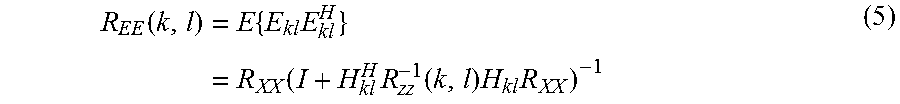
[0057] The QAM symbols could be considered to reside in the Delay-Doppler domain. Thus, time-frequency domain equalization can be shown to be sub-optimal. To see this, consider the residual error after LMMSE filtering, E.sub.kl={circumflex over (X)}.sub.kl.sup.MMSE-X.sub.kl, where E.sub.kl.di-elect cons..sup.N.sup.l. The corresponding MSE matrix R.sub.EE(k,l).di-elect cons..sup.N.sup.l.sup..times.N.sup.l is given by
R EE ( k , l ) = E { E kl E kl H } = R XX ( I + H kl H R zz - 1 ( k , l ) H kl R XX ) - 1 ( 5 ) ##EQU00004##
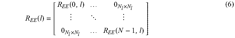
[0058] Since the equalization is performed independently at each time-frequency index, the covariance matrix is independent across the time-frequency grid. For time index l the error covariance matrix is a block diagonal matrix where each entry on the diagonal is an N.sub.l.times.N.sub.l matrix, i.e.
R EE ( l ) = [ R EE ( 0 , l ) 0 N l .times. N l 0 N l .times. N l R EE ( N - 1 , l ) ] ( 6 ) ##EQU00005##
[0059] After linear equalization the channel model expression becomes
{circumflex over (X)}.sub.l.sup.MMSE=X.sub.l+E.sub.l (7)
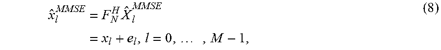
[0060] As the DSFT operation can be decomposed into two one-dimensional DFT transforms, we start by considering a length N IDFT along the frequency axis to the delay domain for OTFS time symbol l. This yields,
x ^ l MMSE = F N H X ^ l MMSE = x l + e l , l = 0 , , M - 1 , ( 8 ) ##EQU00006##
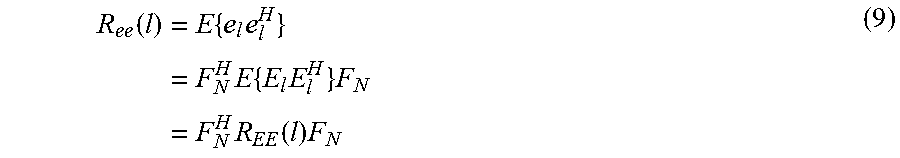
[0061] Where the equalities that x.sub.l=F.sub.NX.sub.l and e.sub.l=F.sub.NE.sub.l are used. The Delay-domain post-equalization error covariance matrix is
R ee ( l ) = E { e l e l H } = F N H E { E l E l H } F N = F N H R EE ( l ) F N ( 9 ) ##EQU00007##
[0062] The DFT transformation in (9) makes R.sub.ee(l) a circulant matrix because R.sub.EE(l) is a diagonal matrix. This also implies that the error covariance matrix is no longer white after transformation to the Delay-domain, i.e. the residual error is correlated. This correlated noise is caused by ISI which can be seen by re-writing (8) as
x l = x ^ l MMSE - e l = F N H G l Y l - e l = A l y l - e l ( 10 ) ##EQU00008##
[0063] where A.sub.l=F.sub.N.sup.HG.sub.lF.sub.N is a circulant matrix. A circulant matrix is characterized by its generator vector, wherein each column of the matrix is a cyclic shift of the generator vector. Let A.sub.l=[a.sub.0,l, . . . , a.sub.N-1,l].sup.T and, without loss of generality, let a.sub.0,l be the generator vector. Then it is straightforward to show that the signal model above describes a cyclic convolution:
x.sub.l(n)=.SIGMA..sub.m=0.sup.N-1a.sub.0,l(m)y.sub.l(n-m).sub.mod N (10A)
[0064] Therefore, ISI is introduced when trying to recover x.sub.1 from its estimate. This same reasoning can be extended from the Delay-time domain to the Delay-Doppler domain by computing the second part of the DSFT, namely, a DFT transformation from the time to Doppler domain. This, in effect is a 2D cyclic convolution that reveals a residual 2D inter-symbol interference across both Delay and Doppler dimensions. In the next section we show how a Decision Feedback Equalizer can be used to suppress this residual ISI.
4. Decision Feedback Equalization
[0065] As the OTFS information symbols reside in the Delay-Doppler domain, where the channel effect on the transmitted signal is a 2D cyclic convolution, a 2D equalizer is desirable at the receiver. One method of implementing a 2D equalizer is as follows. In a first step, a linear equalizer is applied in the time-frequency domain--as described in the previous section. As a second step, a feedback filter is applied in the Delay-Doppler domain to mitigate the residual interference across both delay and Doppler axes. However, since the OTFS block transmission is cyclic, the residual ISI on a particular QAM symbol is caused by other QAM symbols across the Delay-Doppler plane in the current N.times.M transmission block. It may be difficult from an implementation perspective to mitigate ISI in a full 2D scheme. The complexity of a 2D feedback filter for a DFE can be reduced by employing a hybrid DFE. Specifically, (1) The feedforward filter is implemented in the time-frequency domain, (2) the feedback filter is implemented in the Delay-time domain, and (3) the estimated symbols are obtained in the Delay-Doppler domain.
[0066] The rationale for this approach is that after the feedforward filtering, the residual ISI in the Delay domain dominates the interference in the Doppler domain. A set of M parallel feedback filters are implemented corresponding to the M time indices in the OTFS block. This document discloses a DFE receiver for a single input multiple output (SIMO) antenna system (which includes the case of a single receive antenna) system and then extends to the more general multiple input multiple output (MIMO) case, where multiple data streams are transmitted.
[0067] 4.1 SIMO-DFE
[0068] The input to the feedback filter is given by (8) where for the SIMO case x.sub.l.di-elect cons..sup.N. A set of M parallel noise-predictive DFE feedback filters are employed in the Delay-time domain. For time index l, the estimation of x.sub.l(n), n=0, . . . , N-1, is based on exploiting the correlation in the residual error. Given the (LMMSE) feedforward output signal
x.sub.l.sup.MMSE(n)=x.sub.l(n)+e.sub.l(n) (10C)
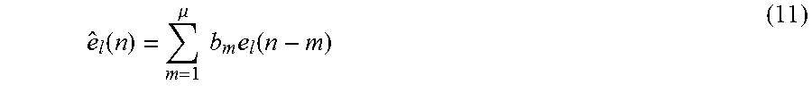
[0069] Some embodiments may be implemented to seek a predicted error signal .sub.l(n) such that the variance of the error term, x.sub.l.sup.MMSE(n)- .sub.l(n) is reduced before estimation. The closer .sub.l(n) is to e.sub.l(n), the more accurate would be the final detection of x.sub.l(n). For simplicity, it may be assumed that the residual error from .mu. past detected symbols is known. Then the predicted error at the nth symbol is given by:
e ^ l ( n ) = m = 1 .mu. b m e l ( n - m ) ( 11 ) ##EQU00009##
[0070] Where {b.sub.m} are the error prediction filter coefficients. For simplicity, the analysis below drops the time index l. The expression above for symbol n can be put in a block processing form by re-writing the error vector at symbol n as .sub.n=[ .sub.n-.mu., .sub.n-.mu.+1, . . . , .sub.n].sup.T. Thus, it can be seen that:
.sub.n=Be.sub.n, (12)
[0071] where B.di-elect cons..sup.(.parallel.+1).times.(.mu.+1) is a strictly lower triangular matrix (i.e. zero entries on the diagonal) with the last row given by b.sub..mu.=[b.sub..mu.,1, . . . , b.sub..mu.,.mu., 0] and e.sub.n=[e.sub.n-.mu., . . . , e.sub.n-1, e.sub.n].sup.T.
[0072] This predictive error formulation depends on the filter length .mu.+1. As such, in some implementations, the pre-feedback error covariance matrix R.sub.ee may be truncated based on this feedback filter length. Taking into account the cyclic (or periodic) nature of (10) the truncated error covariance matrix for symbol n is given by the sub-matrix:
R ~ ee = trunc { R ee } = R ee [ ( n - .mu. , , n ) mod N , ( n - .mu. , , n ) mod N ] ( 13 ) ##EQU00010##
[0073] The final DFE output is then given by
{circumflex over (x)}.sup.DFE(n)={circumflex over (x)}.sup.MMSE(n)-b.sub..mu.e.sub.n,n=0, . . . ,N-1 (14)
[0074] Typically, past residual errors are unknown because the receiver only has access to the output of the feedforward equalizer output {circumflex over (x)}.sup.MMSE(n), n=0, . . . , N-1. Assuming that past hard decisions {circumflex over (x)}.sup.h(n-.mu.), . . . , {circumflex over (x)}.sup.h(n-1)} are correct, some implementations can form an estimate of (n-i) as:
(n-i)={circumflex over (x)}.sup.MMSE(n-i)-{circumflex over (x)}.sup.h(n-i),i=1, . . . ,.mu. (15)
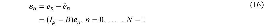
[0075] This document also discloses how reliable past decisions can be obtained. The residual error at the output of the feedback filter is then given by:
n = e n - e ^ n = ( I .mu. - B ) e n , n = 0 , , N - 1 ( 16 ) ##EQU00011##
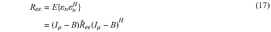
[0076] The resulting error covariance matrix is:
R = E { n n H } = ( I .mu. - B ) R ~ ee ( I .mu. - B ) H ( 17 ) ##EQU00012##
[0077] The Cholesky decomposition of {tilde over (R)}.sub.ee is:
{tilde over (R)}.sub.ee=LDU
[0078] where L is a lower triangular matrix with unity diagonal entries, D is a diagonal matrix with positive entries and U=L.sup.H is an upper triangular matrix. Substituting this decomposition into (17), it is straightforward to show that the post DFE error covariance is minimized if
L.sup.-1=I.sub..mu.-B (18)
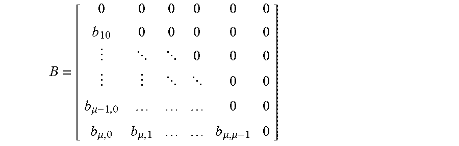
[0079] Where B is a strictly lower triangular matrix
B = [ 0 0 0 0 0 0 b 10 0 0 0 0 0 0 0 0 0 0 b .mu. - 1 , 0 0 0 b .mu. , 0 b .mu. , 1 b .mu. , .mu. - 1 0 ] ##EQU00013##
[0080] FIG. 4 is a block diagram of an example embodiment of a DFE receiver for a SIMO system. For each time slice l.di-elect cons.{0, . . . , M-1} the feedback section works on each sample n .di-elect cons.{0, . . . , N-1}. It can be seen in FIG. 4 that the feedback filter 402 works in parallel across each time slice l=0, . . . , M-1. The Delay-time DFE output is transformed to the Delay-Doppler domain and sent to the soft QAM demodulator (soft slicer), which produces log likelihood ratios (LLRs) as soft input to the FEC decoder.
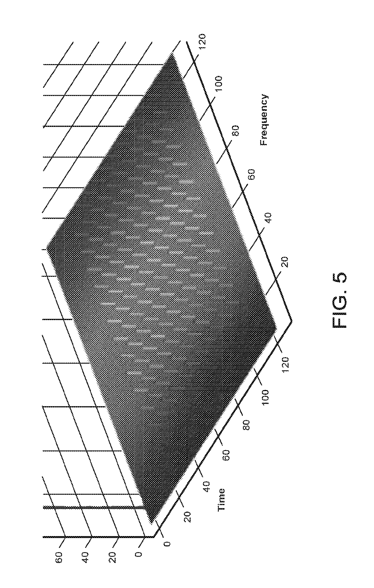
[0081] To start the feedback at n=0, the past symbols {n-.mu., . . . , n-1} are actually modulo N, i.e. they are the last portion of the length N data block, for which hard decisions are not yet available. In some embodiments, a hard decision is made on the output of the feedforward filter. Alternatively or additionally, in some embodiments, a known sequence is appended at the end of each transmitted block, which also helps mitigate error propagation. For example, data and pilot regions may be multiplexed in the Delay-Doppler domain as shown in the example graph in FIG. 5. Here, the pilot region consists of a single impulse at (0, 0) and a zero-power region at the edges of the data region to facilitate estimation of the Delay-Doppler channel response at the receiver. This pilot region constitutes a known sequence that can be used to start the feedback filter.
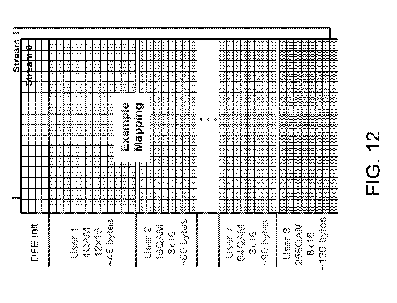
[0082] In some embodiments, the transmitted signals may include a frame structure in which the lowest constellations are sent at the top (beginning) of a frame, in the delay domain. FIG. 12 show an example of multiplexing information bits for different users in a transmission on a stream-basis such that a pilot signal transmission portion may be at the beginning of the transmission frame, followed by the lowest modulation (4QAM, in this case), followed by increasing modulation for different users based on the channel condition to the corresponding user equipment. The data being sent to different users may thus be arranged along the delay dimension.
[0083] As shown the example of FIG. 12, the transmitted wireless signal may include one or more streams (spatial layers). Each stream may include a first portion that includes a decision feedback equalization signal, followed by a second portion in which data being transmitted (e.g., modulation information bits) to multiple user equipment is arranged in increasing level of modulation constellation density along the delay dimension.
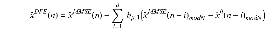
[0084] In some implementations, the DFE algorithm may be described as follows: (1) Compute the time-frequency LMMSE (feedforward) equalizer output. (2) For the 1.sup.th OTFS symbol, transform the LMMSE equalizer output to Delay-time domain to obtain (8). (3) Compute the delay-domain error covariance matrix R.sub.ee(l)=F.sub.N.sup.HR.sub.EE(l)F.sub.N. In some implementation, rather than performing the full matrix multiplications, a faster method may be used. (4) Computing the truncated error covariance matrix in (13). (5) Obtaining the filter b.sub..mu. as the last row of B=I.sub..mu.-L.sup.-1. (6) DFE output for sample n is
x ^ DFE ( n ) = x ^ MMSE ( n ) - i = 1 .mu. b .mu. , 1 ( x ^ MMSE ( n - i ) mod N - x ^ h ( n - i ) mod N ) ##EQU00014##
[0085] (6) Collecting all time slices and transform to the Delay-Doppler domain.
[0086] 4.2 MIMO-DFE
[0087] In some embodiments, a MIMO DFE technique could be largely based on the SIMO case but with some differences. First, the expressions in the SIMO case still hold but with the difference that each element of a vector or matrix is now of dimension N.sub.l. For instance each element of the (.mu.+1).times.(.mu.+1) covariance matrix of (13) is an N.sub.l.times.N.sub.l matrix. Second, while the cancellation of past symbols eliminates, or at least mitigates, the ISI, there is still correlation between the MIMO streams. It can be shown that, by design, the noise-predictive MIMO DFE structure also performs successive inter-stream interference cancellation (SIC). In the present case, the cancellation between streams may be ordered or un-ordered. This document describes both these cases separately and shows an extension of the DFE receiver to incorporate a near maximum likelihood mechanism.
[0088] 4.3 MIMO DFE with SIC
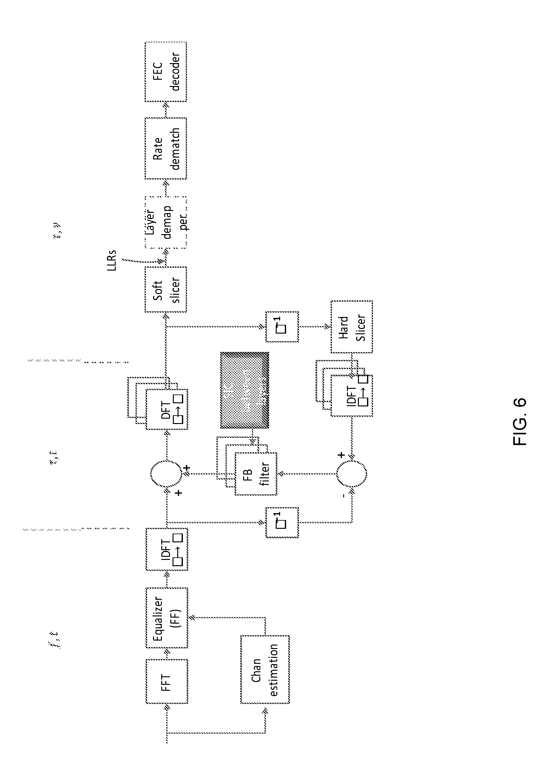
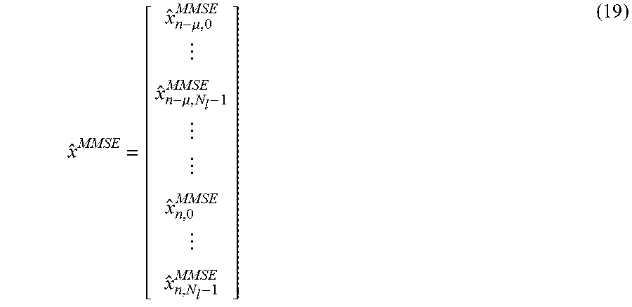
[0089] FIG. 6 depicts an example embodiment of a MIMO DFE receiver. The LMMSE feedforward output {circumflex over (x)}.sup.MMSE(n) is a vector of dimension N.sub.l>1. Similarly to the SIMO (N.sub.l=1) case, the MIMO DFE works in parallel across the time axis. For convenience, the time index l=0, . . . , M-1 are omitted. To detect the data vector at the nth delay index x.sub.n for any time index, arrange the observation vector from the feedforward filter output of (8) first according to spatial layers and then according to the delay domain as:
x ^ MMSE = [ x ^ n - .mu. , 0 MMSE x ^ n - .mu. , N l - 1 MMSE x ^ n , 0 MMSE x ^ n , N l - 1 MMSE ] ( 19 ) ##EQU00015##
[0090] The frequency-domain error covariance matrix of (6) is a block diagonal matrix, where each diagonal element R.sub.EE(n,n).di-elect cons..sup.N.sup.l.sup..times.N.sup.l. Define the block N.times.N DFT matrix as
{tilde over (F)}.sub.N=F.sub.NI.sub.N.sub.l (20)
[0091] Then, it is straightforward to show that the corresponding delay-domain error covariance is given by:
R.sub.ee={tilde over (F)}.sub.N.sup.HR.sub.EE{tilde over (F)}.sub.N (21)
[0092] Similar to the SIMO case, the columns of R.sub.ee an be obtained by an N.sub.l.times.N.sub.l block circular shift of the generator vector R.sub.ee[0].di-elect cons..sup.NN.sup.l.sup..times.N.sup.l.
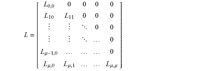
[0093] Again, implementations can obtain the truncated covariance matrix of (13), and after Cholesky decomposition, the lower triangular matrix is of the form:
L = [ L 0 , 0 0 0 0 0 L 10 L 11 0 0 0 0 0 0 L .mu. - 1 , 0 0 L .mu. , 0 L .mu. , 1 L .mu. , .mu. ] ##EQU00016##
[0094] Each diagonal entry of L is an N.sub.l.times.N.sub.l lower triangular matrix. The feedback filter is taken as the last block row of the B matrix obtained as in (18) but now for the MIMO case. Hence, the matrix feedback filter b.sub..mu..di-elect cons..sup.N.sup.l.sup..times.N.sup.l.sup.(.mu.+1) is given by:
b.sub..mu.=[b.sub..mu.,0,b.sub..mu.,1, . . . ,b.sub..mu.,.mu.] (22)
[0095] The last block element b.sub..mu.,.mu. is strictly lower triangular. To see the effect of the inter-stream cancellation, consider the 2.times.2 case. The last block element of the feedback filter is given by
b .mu. , .mu. = [ 0 0 .alpha. 0 ] ( 23 ) ##EQU00017##
[0096] From (19) the current symbol vector to be detected is x.sub.n=[x.sub.n,0 x.sub.n,1].sup.T. From the product b.sub..mu.,.mu.e.sub.n which is performed in (14) it can be seen that for the feedback filter does not act on the error in the first layer, while for the second layer, there is a filter coefficient acting on the first layer.
[0097] The interpretation may be as follows: for the first layer a prediction error is computed only from hard decisions of past symbol vectors. For the second layer, the detection of the first layer is used to predict error for detecting the second layer. More generally, detection of a spatial layer for a current symbol vector utilizes hard decisions from past detected symbol vectors as well as hard decisions for preceding layers in the current symbol. This is equivalently an SIC mechanism without any ordering applied to the stream cancellation. A different method is to apply ordering across the spatial layers in the MIMO system in scenarios where the SINR statistics are not identical across spatial layers.
[0098] 4.4 MIMO DFE with Maximum Likelihood Detection
[0099] A different method to the DFE is to only cancel the ISI from past symbol vectors. That is, to detect x.sub.n, implementations can use an observation vector of v.sub.n,past=[v.sub.n-.mu..sup.T, v.sub.n-.mu.-1.sup.T, . . . , v.sub.n-1.sup.T].sup.T to form the prediction error vector for (14). If the cancellation of ISI is perfect, the post DFE signal expression for the n.sup.th symbol vector
{circumflex over (x)}.sub.n.sup.DFE=x.sub.n+e.sub.n (24)
[0100] is now similar to what is expected in say OFDM, where the interference is only between the spatial layers (or streams). Therefore, implementations can apply a maximum likelihood receiver to detect the QAM symbols on each layer.
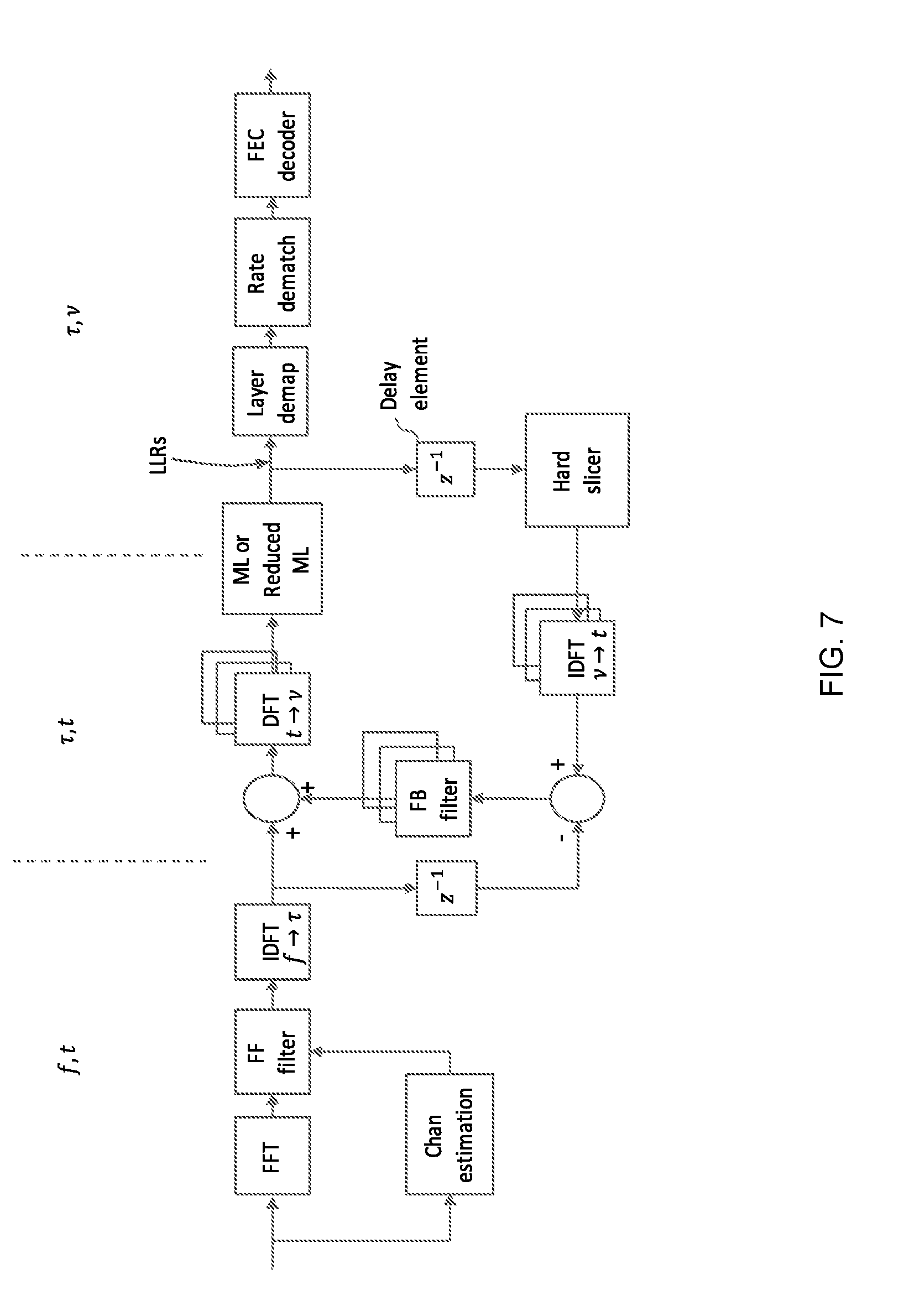
[0101] FIG. 7 depicts an example embodiment of a DFE-ML receiver, where a hard slicer is applied for the input to the DFE feedback path. Given a QAM constellation .OMEGA., the ML decision is
x n ML = arg max u .di-elect cons. .OMEGA. N l ( u - x ^ n DFE ) H R ee - 1 ( u - x ^ n DFE ) ( 25 ) ##EQU00018##
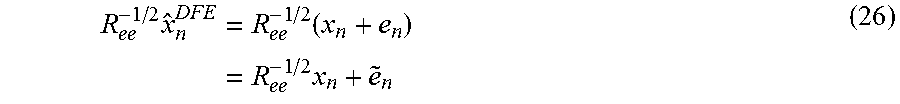
[0102] The error covariance matrix, R.sub.ee corresponds to the additive error in (24) that is obtained after cancelling interference from past symbols. Furthermore, R.sub.ee is not white. To improve detection performance, some embodiments may first whiten the ML receiver input as follows. First, decompose the error covariance matrix as R.sub.ee=R.sub.ee.sup.1/2R.sub.ee.sup.T/2. Then, let the input to the ML receiver be
R ee - 1 / 2 x ^ n DFE = R ee - 1 / 2 ( x n + e n ) = R ee - 1 / 2 x n + e ~ n ( 26 ) ##EQU00019##
[0103] This expression now follows the basic MIMO equation for ML, i.e. y=Hx+n, where, in our case, the channel H=R.sub.ee.sup.-1/2x.sub.n and the noise covariance matrix E{{tilde over (e)}.sub.n{tilde over (e)}.sub.n.sup.H}=I.sub.N.sub.l.
[0104] In addition, the ML provides a log likelihood ratio (LLR) for each transmitted bit. Rather than resort to hard QAM decisions for the DFE, a different method is to generate soft QAM symbols based on the LLR values from the ML receiver.
[0105] FIG. 8 illustrates an example embodiment of a DFE-ML receiver with soft input to the feedback path. While all other functional blocks are similar to FIG. 7, in place of a hard slicer, a soft QAM modulator may be used to provide input to the IDFT operation in the feedback path.
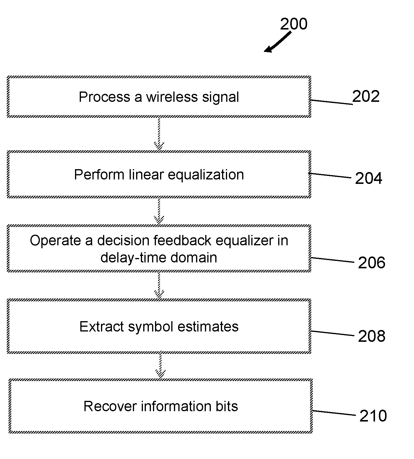
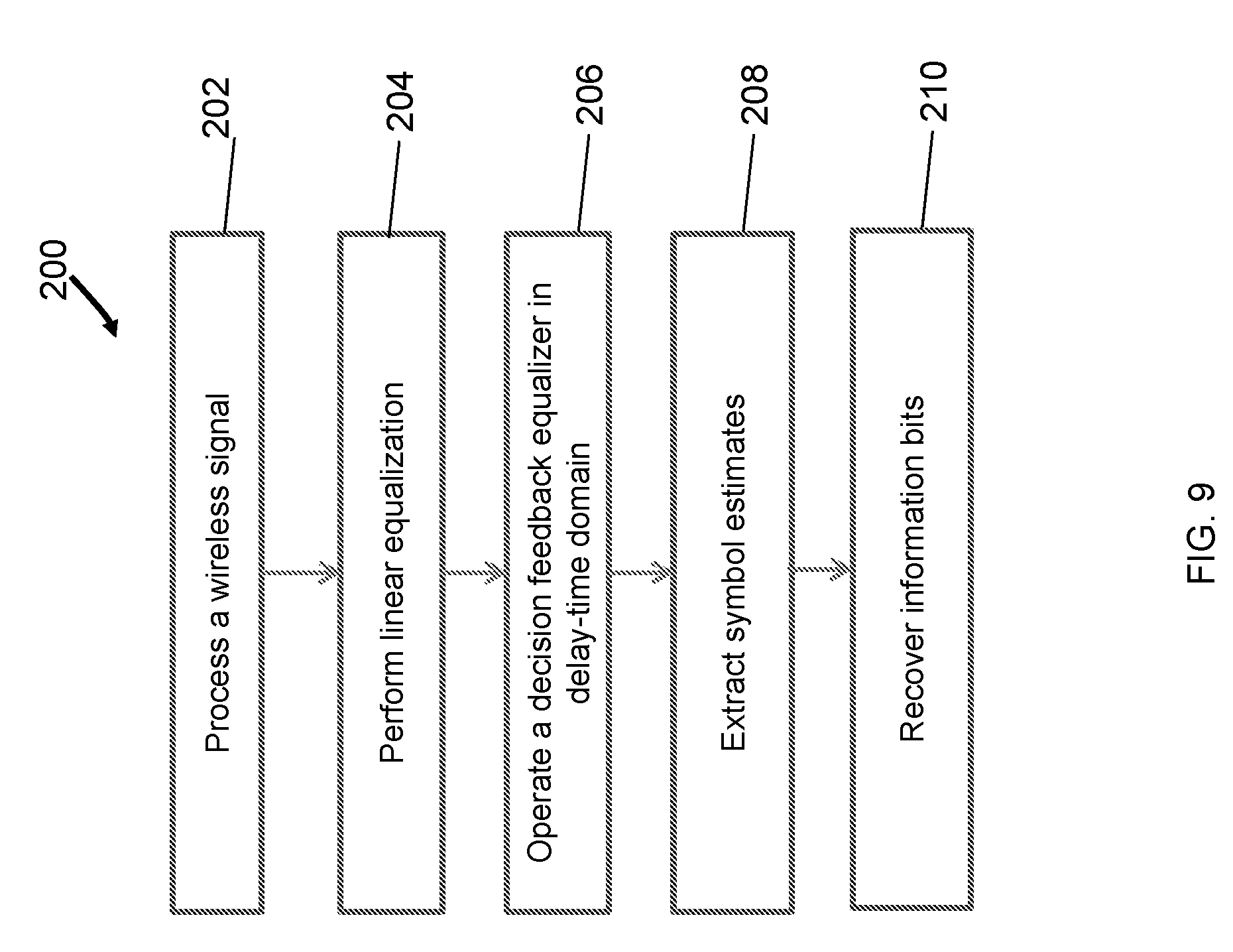
[0106] FIG. 9 is a flowchart for an example method 200 of wireless communication. The method 200 may be implemented by a wireless receiver, e.g., receiver 102 depicted in FIG. 1.
[0107] The method 200 includes, at 202, processing a wireless signal comprising information bits modulated using an OTFS modulation scheme to generate time-frequency domain digital samples. In some embodiments, the time-frequency domain samples may be generated by applying a two-dimensional transform to the wireless signal. The two-dimensional transform may be, for example, a discrete Symplectic Fourier transform. In some embodiments, the two-dimensional transform may be applied by windowing over a grid in the time-frequency domain.
[0108] In some embodiments, the processing 202 may be performed using an RF front end which may downcovert the received signal from RF to baseband signal. Automatic Gain Control may be used to generate an AGC-corrected baseband signal. This signal may be digitized by an analog to digital converter to generate digital samples.
[0109] The method 200 includes, at 204, performing linear equalization of the time-frequency domain digital samples resulting in an equalized signal. Various embodiments of linear equalization are described in this document. In some embodiments, the linear equalization may be performed using a mean square error criterion and minimizing the error. Some examples are given with reference to Eq. (4) to Eq. (9). In some embodiments, a Wiener filtering formulation may be used for the optimization.
[0110] The method 200 further includes, at 206, inputting the equalized signal to a feedback filter operated in a delay-time domain to produce a decision feedback equalizer (DFE) output signal. Various possibilities of DFE include single-input, multiple output (SIMO) DFE (Section 4.1), multiple-input multiple-output (MIMO) DFE (Section 4.2), MIMO-DFE with successive interference cancellation (Section 4.3), and MIMO DFE with maximum likelihood estimation (Section 4.4), as described herein.
[0111] The method 200 further includes, at 208, extracting symbol estimates from the DFE output signal. As described with reference to FIGS. 2-4 and 6-8, in some embodiments, the extraction operation may be performed in the delay-Doppler domain.
[0112] The method 200 further includes, at 210, recovering the information bits from the symbol estimates. The symbols may be, for example, quadrature amplitude modulation symbols such as 4, 8, 16 or higher QAM modulation symbols.
[0113] In some embodiments, a wireless signal transmission method may include generating data frames, e.g., as depicted in FIG. 12, and transmitting the generated data frames to multiple UEs over a wireless communication channel. For example, the transmission method may be implemented at a base station in a wireless network.
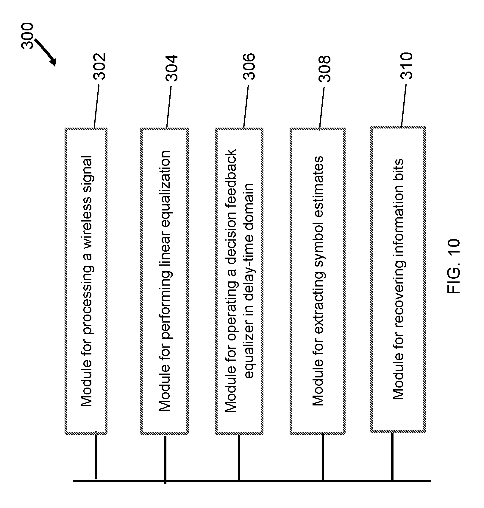
[0114] FIG. 10 is a block diagram showing an example communication apparatus 300 that may implement the method 200. The apparatus 300 includes a module 302 for processing a wireless signal received at one or more antennas of the apparatus 300. A module 304 may perform linear equalization in the time-frequency domain. The module 306 may perform DFE operation in the delay-time domain. The module 308 may perform symbol estimation in the delay-Doppler domain. The module 310 may recover information bits from modulated symbols.
[0115] FIG. 11 shows an example of a wireless transceiver apparatus 600. The apparatus 600 may be used to implement method 200. The apparatus 600 includes a processor 602, a memory 604 that stores processor-executable instructions and data during computations performed by the processor. The apparatus 600 includes reception and/or transmission circuitry 606, e.g., including radio frequency operations for receiving or transmitting signals.
[0116] It will be appreciated that techniques for wireless data reception are disclosed using two-dimensional reference signals based on delay-Doppler domain representation of signals.
[0117] The disclosed and other embodiments, modules and the functional operations described in this document can be implemented in digital electronic circuitry, or in computer software, firmware, or hardware, including the structures disclosed in this document and their structural equivalents, or in combinations of one or more of them. The disclosed and other embodiments can be implemented as one or more computer program products, i.e., one or more modules of computer program instructions encoded on a computer readable medium for execution by, or to control the operation of, data processing apparatus. The computer readable medium can be a machine-readable storage device, a machine-readable storage substrate, a memory device, a composition of matter effecting a machine-readable propagated signal, or a combination of one or more them. The term "data processing apparatus" encompasses all apparatus, devices, and machines for processing data, including by way of example a programmable processor, a computer, or multiple processors or computers. The apparatus can include, in addition to hardware, code that creates an execution environment for the computer program in question, e.g., code that constitutes processor firmware, a protocol stack, a database management system, an operating system, or a combination of one or more of them. A propagated signal is an artificially generated signal, e.g., a machine-generated electrical, optical, or electromagnetic signal, that is generated to encode information for transmission to suitable receiver apparatus.
[0118] A computer program (also known as a program, software, software application, script, or code) can be written in any form of programming language, including compiled or interpreted languages, and it can be deployed in any form, including as a standalone program or as a module, component, subroutine, or other unit suitable for use in a computing environment. A computer program does not necessarily correspond to a file in a file system. A program can be stored in a portion of a file that holds other programs or data (e.g., one or more scripts stored in a markup language document), in a single file dedicated to the program in question, or in multiple coordinated files (e.g., files that store one or more modules, sub programs, or portions of code). A computer program can be deployed to be executed on one computer or on multiple computers that are located at one site or distributed across multiple sites and interconnected by a communication network.
[0119] The processes and logic flows described in this document can be performed by one or more programmable processors executing one or more computer programs to perform functions by operating on input data and generating output. The processes and logic flows can also be performed by, and apparatus can also be implemented as, special purpose logic circuitry, e.g., an FPGA (field programmable gate array) or an ASIC (application specific integrated circuit).
[0120] Processors suitable for the execution of a computer program include, by way of example, both general and special purpose microprocessors, and any one or more processors of any kind of digital computer. Generally, a processor will receive instructions and data from a read only memory or a random access memory or both. The essential elements of a computer are a processor for performing instructions and one or more memory devices for storing instructions and data. Generally, a computer will also include, or be operatively coupled to receive data from or transfer data to, or both, one or more mass storage devices for storing data, e.g., magnetic, magneto optical disks, or optical disks. However, a computer need not have such devices. Computer readable media suitable for storing computer program instructions and data include all forms of non-volatile memory, media and memory devices, including by way of example semiconductor memory devices, e.g., EPROM, EEPROM, and flash memory devices; magnetic disks, e.g., internal hard disks or removable disks; magneto optical disks; and CD ROM and DVD-ROM disks. The processor and the memory can be supplemented by, or incorporated in, special purpose logic circuitry.
[0121] While this patent document contains many specifics, these should not be construed as limitations on the scope of an invention that is claimed or of what may be claimed, but rather as descriptions of features specific to particular embodiments. Certain features that are described in this document in the context of separate embodiments can also be implemented in combination in a single embodiment. Conversely, various features that are described in the context of a single embodiment can also be implemented in multiple embodiments separately or in any suitable sub-combination. Moreover, although features may be described above as acting in certain combinations and even initially claimed as such, one or more features from a claimed combination can in some cases be excised from the combination, and the claimed combination may be directed to a sub-combination or a variation of a sub-combination. Similarly, while operations are depicted in the drawings in a particular order, this should not be understood as requiring that such operations be performed in the particular order shown or in sequential order, or that all illustrated operations be performed, to achieve desirable results.
[0122] Only a few examples and implementations are disclosed. Variations, modifications, and enhancements to the described examples and implementations and other implementations can be made based on what is disclosed.
* * * * *
D00000
D00001
D00002
D00003
D00004
D00005
D00006
D00007
D00008
D00009
D00010
D00011
D00012


P00001

P00002

XML
uspto.report is an independent third-party trademark research tool that is not affiliated, endorsed, or sponsored by the United States Patent and Trademark Office (USPTO) or any other governmental organization. The information provided by uspto.report is based on publicly available data at the time of writing and is intended for informational purposes only.
While we strive to provide accurate and up-to-date information, we do not guarantee the accuracy, completeness, reliability, or suitability of the information displayed on this site. The use of this site is at your own risk. Any reliance you place on such information is therefore strictly at your own risk.
All official trademark data, including owner information, should be verified by visiting the official USPTO website at www.uspto.gov. This site is not intended to replace professional legal advice and should not be used as a substitute for consulting with a legal professional who is knowledgeable about trademark law.