Method for Determining Spacing of Hydraulic Fractures in a Rock Formation
Roussel; Nicolas P. ; et al.
U.S. patent application number 13/531031 was filed with the patent office on 2012-12-27 for method for determining spacing of hydraulic fractures in a rock formation. Invention is credited to Nicolas P. Roussel, Mukul M. Sharma.
| Application Number | 20120325462 13/531031 |
| Document ID | / |
| Family ID | 47360733 |
| Filed Date | 2012-12-27 |


View All Diagrams
| United States Patent Application | 20120325462 |
| Kind Code | A1 |
| Roussel; Nicolas P. ; et al. | December 27, 2012 |
Method for Determining Spacing of Hydraulic Fractures in a Rock Formation
Abstract
Methods of the present disclosure include determining an expected trajectory of induced fractures in a rock formation, analyzing net pressure associated with the induced fractures, and determining at least one of spacing of induced fractures and a property of the induced fractures based on the net pressure. Computer-readable medium containing the method are also disclosed. Other related methods are also disclosed.
| Inventors: | Roussel; Nicolas P.; (Houston, TX) ; Sharma; Mukul M.; (Austin, TX) |
| Family ID: | 47360733 |
| Appl. No.: | 13/531031 |
| Filed: | June 22, 2012 |
Related U.S. Patent Documents
| Application Number | Filing Date | Patent Number | ||
|---|---|---|---|---|
| 61501003 | Jun 24, 2011 | |||
| Current U.S. Class: | 166/250.1 |
| Current CPC Class: | G01V 2210/624 20130101; E21B 43/26 20130101; G01V 1/306 20130101 |
| Class at Publication: | 166/250.1 |
| International Class: | E21B 49/00 20060101 E21B049/00 |
Goverment Interests
GOVERNMENT LICENSE RIGHTS
[0002] This invention was made with government support under DE-AC26-07NT42677 awarded by The Department of Energy. The United States Government has certain rights in the invention.
Claims
1. A method comprising: determining an expected trajectory of induced fractures; analyzing net pressure associated with the induced fractures; and determining at least one of spacing of induced fractures and a property of the induced fractures based on the net pressure.
2. The method of claim 1, wherein determining an expected trajectory of induced factures comprises: analyzing stresses prior to inducing fracturing; modeling a trajectory of a first fracture; determining effects on the stresses based on the modeled trajectory of the first fracture; and modeling a trajectory of a subsequent fracture based on the effects on the stresses caused by the first fracture.
3. The method of claim 2, further comprising decreasing the spacing of induced fractures based at least on the modeling of the first and subsequent fractures.
4. The method of claim 1, further comprising determining a maximum horizontal stress.
5. The method of claim 1, wherein the property of the induced fractures includes an expected trajectory of a subsequently induced fracture.
6. The method of claim 1, wherein the net pressure is determined by at least one of surface pressures or down-hole pressures during fracturing.
7. A method of optimizing fracture spacing comprising: propagating an initial fracture; measuring pressure associated with propagating the initial fracture; determining a minimum spacing required to prevent a second fracture from intersecting the initial fracture; and propagating the second fracture at least the minimum spacing distance away from the initial fracture.
8. The method of optimizing fracture spacing of claim 7, further comprising: measuring pressure associated with propagating the second fracture; determining a second minimum spacing required to prevent a third fracture from intersecting the second fracture; and propagating the third fracture at least the second minimum spacing distance away from the second fracture.
9. The method of optimizing fracture spacing of claim 8, wherein determining the second minimum spacing is based at least on the pressure associated with propagating the second fracture.
10. The method of optimizing fracture spacing of claim 7, wherein the second fracture is propagated at a distance sufficient to allow a third fracture to be propagated between the first and the second fractures.
11. The method of optimizing fracture spacing of claim 10, further comprising: determining spacing required to prevent the third fracture from intersecting the first and second fractures based at least on the pressure associated with propagating the first and the second fractures; and determining a decreased distance between a fourth and the second fracture based at least on the spacing required to prevent the third fracture intersecting the first and second fractures and the pressure associated with propagating the second fracture.
12. The method of optimizing fracture spacing of claim 7, wherein determining the minimum spacing comprises: modeling stresses caused by the first fracture based at least on the pressure associated with propagating the first fracture; and modeling a trajectory of the second fracture based on the modeled stresses.
13. The method of optimizing fracture spacing of claim 7, wherein determining the minimum spacing comprises modeling at least one of an attraction zone and a repulsion zone associated with the first fracture based at least on net pressure, in-situ stress contrast, or average angle of deviation from a trajectory of the first fracture.
14. The method of optimizing fracture spacing of claim 13, wherein the minimum spacing is outside of the attraction zone associated with the first fracture.
15. The method of optimizing fracture spacing of claim 13, wherein determining the minimum spacing further comprises modeling a stress reversal region.
16. A method of optimizing fracture spacing comprising: analyzing stresses associated with a first set of at least one fractures associated with a first well; analyzing stresses associated with a second set of at least one fractures associated with a second well; and determining spacing of a fracture associated with a third well such that the fracture associated with the third well does not intersect with the first set and the second set of fractures, the third well running between the first and second wells.
17. The method of optimizing fracture spacing of claim 16, wherein determining spacing of the fracture associated with the third well comprises: modeling the stresses associated with the first and the second set of fractures; modeling a trajectory of the fracture associated with the third well.
18. The method of optimizing fracture spacing of claim 16, wherein analyzing stresses associated with the first set of at least one fractures is based at least on net pressure of propagating the first set of at least one fractures.
19. The method of optimizing fracture spacing of claim 16, wherein the first set and the second set of fractures comprise at least two fractures and are spaced such that the fracture associated with the third well is substantially between a first and a second fracture of the first set of fractures and between a first and a second fracture of the second set of fractures.
20. The method of optimizing fracture spacing of claim 19, further comprising determining a decreased distance between a third and the second fracture of the first set of fractures and a third and the second fracture of the second set of fractures based at least on the spacing required to prevent the fracture associated with the third well from intersecting the first and the second set of fractures, the distance determined such that a second fracture associated with the third well may be propagated between the second and the third fractures of the first set of fractures and the second and the third fractures of the second set of fractures without intersecting the first or the second set of fractures.
21. A method of determining maximum horizontal pressure comprising: measuring an actual pressure during each stage of fracturing of a rock formation; determining a theoretical expected pressure during each stage of fracturing of the rock formation; determining a maximum horizontal pressure of the rock formation based at least on a comparison of the theoretical expected pressure and the measured actual pressure.
Description
RELATED APPLICATION
[0001] This application claims benefit under 35 U.S.C. .sctn.119(e) of U.S. Provisional Application Ser. No. 61/501,003, entitled "METHOD FOR DETERMINING SPACING OF HYDRAULIC FRACTURES IN A ROCK FORMATION," filed Jun. 24, 2011, the entire content of which is incorporated herein by reference.
TECHNICAL FIELD
[0003] The present disclosure relates in general to well drilling and, more particularly, to a method for determining spacing of hydraulic fractures in a rock formation.
BACKGROUND
[0004] Hydrocarbon (e.g., oil, natural gas, etc.) reservoirs may be found in geologic formations that have little to no porosity (e.g., shale, sandstone etc.). The hydrocarbons may be trapped within fractures and pore spaces of the formation. Additionally, the hydrocarbons may be adsorbed onto organic material of the shale formation. The rapid development of extracting hydrocarbons from these unconventional reservoirs can be tied to the combination of horizontal drilling and hydraulic fracturing ("fracing") of the formations. Horizontal drilling has allowed for drilling along and within hydrocarbon reservoirs of a formation to better capture the hydrocarbons trapped within the reservoirs. Additionally, more hydrocarbons may be captured by increasing the number of fractures in the formation and/or increasing the size of already present fractures through fracing. The spacing between fractures as well as the ability to stimulate the fractures naturally present in the rock may be major factors in the success of horizontal completions in unconventional hydrocarbon reservoirs.
SUMMARY
[0005] In one embodiment, a method is disclosed comprising determining an expected trajectory of induced fractures, analyzing net pressure associated with the induced fractures, and determining at least one of spacing of induced fractures and a property of the induced fractures based on the net pressure. Computer-readable medium containing the same are also disclosed.
[0006] In an alternative embodiment, a method of optimizing fracture spacing is disclosed. The method includes propagating an initial fracture, measuring pressure associated with propagating the initial fracture, determining a minimum spacing required to prevent a second fracture from intersecting the initial fracture, and propagating the second fracture at least the minimum spacing distance away from the initial fracture.
[0007] In other embodiments, also disclosed is a method of optimizing fracture spacing. The method includes analyzing stresses associated with a first set of at least one fractures associated with a first well, analyzing stresses associated with a second set of at least one fractures associated with a second well, and determining spacing of a fracture associated with a third well such that the fracture associated with the third well does not intersect with the first set and the second set of fractures, the third well running between the first and second wells.
[0008] In still other embodiments, also disclosed is a method of determining maximum horizontal pressure. The method includes measuring an actual pressure during each stage of fracturing of a rock formation, determining a theoretical expected pressure during each stage of fracturing of the rock formation, and determining a maximum horizontal pressure of the rock formation based at least on a comparison of the theoretical expected pressure and the measured actual pressure.
BRIEF DESCRIPTION OF THE DRAWINGS
[0009] FIG. 1 illustrates an example schematic of a gas well configured to extract natural gas from a gas rich shale formation, according to some embodiments of the present disclosure;
[0010] FIGS. 2a and 2b illustrate examples of the reorientation of stresses in a rock formation due to the placement of a fracture orthogonal to a horizontal well according to some embodiments of the present disclosure;
[0011] FIG. 3 illustrates the geometry of a single transverse fracture of a shale formation that includes a pay zone that may include hydrocarbons (e.g., natural gas) and bounding layers that may bound the pay zone, according to some embodiments of the present disclosure;
[0012] FIG. 4 illustrates a three dimensional model of multiple transverse fractures in a layered rock formation according to some embodiments of the present disclosure;
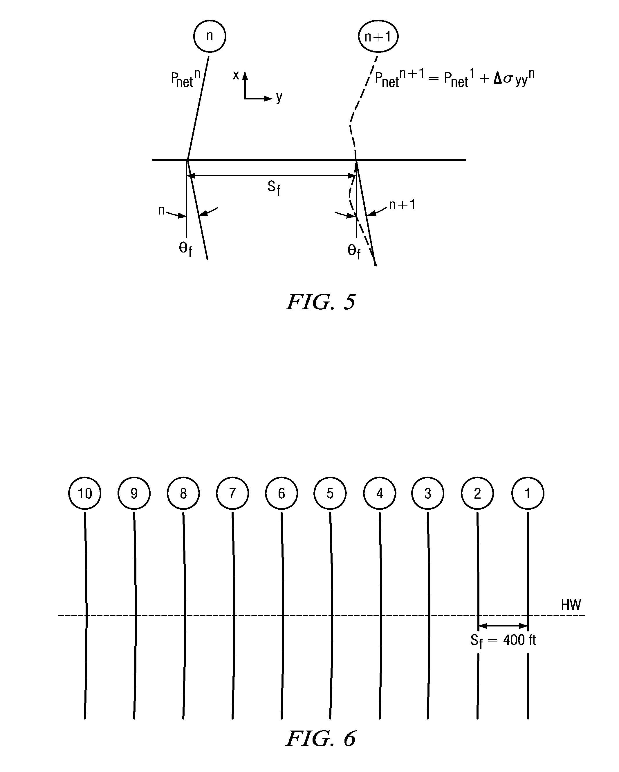
[0013] FIG. 5 illustrates the calculated propagation of a subsequent fracture (n+1) based on the mechanical stress interference of a previous fracture (n), according to some embodiments of the present disclosure;
[0014] FIG. 6 illustrates the results of calculating fracture propagation with each fracture spaced approximately 400 feet apart, according to some embodiments of the present disclosure;
[0015] FIG. 7 illustrates the results of calculating fracture propagation with each fracture spaced approximately 300 feet apart, according to some embodiments of the present disclosure;
[0016] FIG. 8 illustrates the stress distribution of a rock formation with the stress distribution being influenced by the propagation of a fracture produced during a fourth stage of a fracture treatment, according to some embodiments of the present disclosure;
[0017] FIG. 9 illustrates fracture propagation with the fracture spacing reduced to 250 ft., according to some embodiments of the present disclosure;
[0018] FIG. 10 illustrates the stress distribution of a rock formation caused by fractures of FIG. 9, according to some embodiments of the present disclosure;
[0019] FIG. 11 illustrates fracture propagation with the fracture spacing reduced to 200 ft., according to some embodiments of the present disclosure;
[0020] FIG. 12 illustrates fracture propagation with the fracture spacing reduced to 150 ft., according to some embodiments of the present disclosure;
[0021] FIGS. 13a and 13b illustrate the impact of fracture spacing on the angle of deviation of the fractures from the orthogonal path, according to some embodiments of the present disclosure;
[0022] FIG. 14 illustrates the impact of fracture spacing on the evolution of the net closure stress, according to some embodiments of the present disclosure;
[0023] FIGS. 15a and 15b illustrate the horizontal stress of a rock formation with a stress reversal region associated with a fracture, according to some embodiments of the present disclosure;
[0024] FIGS. 16a and 16b illustrate the differences between performing consecutive fracturing and alternate fracturing, according to some embodiments of the present disclosure;
[0025] FIGS. 17a and 17b illustrate the stress orientation of a rock formation with stress reversal regions associated with a first fracture and a second fracture, according to some embodiments of the present disclosure;
[0026] FIG. 18 shows a spacing of fractures for which the stress contrast may be lowest, according to some embodiments of the present disclosure;
[0027] FIG. 19 illustrates that the deviatoric stress may approach zero in a near wellbore region in the case of optimum spacing in an alternate fracturing sequence, according to some embodiments of the present disclosure;
[0028] FIG. 20 illustrates an example of fracture spacing that may be done with multiple horizontal lateral wells, according to some embodiments of the present disclosure;
[0029] FIGS. 21a and 21b illustrate the stress distribution between two pairs of fractures propagated from outside lateral wells, according to some embodiments of the present disclosure;
[0030] FIG. 22 illustrates the relationship between the length of a "middle fracture" propagating from a center lateral well for different values of the fracture length with respect to the inter-well spacing, according to some embodiments of the present disclosure; and
[0031] FIG. 23 illustrates the local stress contrast that may be recorded along the assumed propagation direction of a middle fracture, according to some embodiments of the present disclosure.
DETAILED DESCRIPTION
[0032] FIG. 1 illustrates an example schematic of a gas well 100 configured to extract natural gas from a gas rich shale formation 102. Well 100 may be drilled using horizontal drilling methods to create a wellbore 104 that runs within and along shale formation 102. In the present example, wellbore 104 may be drilled such that wellbore 104 runs perpendicular to the maximum horizontal in-situ stresses of shale formation 102 to obtain better production of well 100.
[0033] Shale formation 102 may produce natural gas that is trapped in fractures and pore spaces of shale formation 102. The natural gas may also be adsorbed in organic material included in the shale of shale formation 102. As well bore 104 runs through shale formation 102, well bore 104 may also run through fractures (not expressly shown) of shale formation 102. The gas in the fractures may enter well bore 104 and may accordingly be retrieved at a drilling rig 106 of well 100. As gas leaves the fractures of shale formation 102, the gas adsorbed on the organic material may be released into the fractures such that the adsorbed gas may also be retrieved. As the number of fractures of shale formation 102 that well bore 104 passes through increases, the amount of gas that may be produced by well 100 may also increase. Therefore, increasing the number of fractures in shale formation 102 along well bore 104 may increase the gas production of well 100.
[0034] The number and/or size of fractures in shale formation 102 may be increased using hydraulic fracturing ("fracing"). Fracing may refer to any process used to initiate and propagate a fracture in a rock formation. Additionally fracing may be used to increase existing fractures in a rock formation. Fracing may include forcing a hydraulic fluid in a fracture of a rock formation to increase the size of the fracture and introducing proppant (e.g., sand) in the newly induced fracture to keep the fracture open. The fracture may be an existing fracture in the formation, or may be initiated using a variety of techniques known in the art. The amount of pressure needed to extend and propagate the fracture may be referred to as the "fracturing pressure."
[0035] As shown in further detail with respect to FIGS. 2a and 2b, producing fractures during fracing may change the stress properties of a rock formation. Accordingly, subsequent transverse fractures initiated from a horizontal well may deviate toward or away from the previous fracture depending on the stress reorientation caused by the fracing. The stress reorientation may be a function of mechanical properties of the reservoir rock, fracture spacing, and the orientation of the previous fracture. As described in further detail below, in some instances spacing frac treatments too close together may result in a subsequent fracture intersecting with a previous fracture. Therefore, in such instances, the contribution of the subsequent fracture in hydrocarbon production may be reduced or minimized.
[0036] As disclosed in further detail below, the spacing of performing fracturing operations for a hydrocarbon well, such as gas well 100, may be determined using net pressure measurements to determine a minimum frac spacing that also reduces the likelihood of subsequent fractures intersecting and interfering with previous fractures. In some instances, net pressure may be determined by surface pressures or down-hole pressures during fracturing. Therefore, the selection of fracture spacing may be such that the number of fractures initiated from a horizontal wellbore may be increased while also reducing the likelihood that the fractures may interfere and/or intersect with each other to allow for better production rates and depletion of hydrocarbons with each induced fracture. Therefore, the economic efficiency of fracturing may be improved and the cost of retrieving hydrocarbons from tight rock formations (e.g., shale formation 102) may be reduced.
[0037] Modifications, additions or omissions may be made to FIG. 1 without departing from the present disclosure. For example, although FIG. 1 is described as performing fracing with respect to a shale gas formation, the present disclosure may be used to improve frac spacing for any suitable formation (e.g., a tight sand formation, coalbed methane, sandstone, limestone, oil shale). Additionally, although well 100 is described as being used to extract natural gas, it is understood that the principles described herein may be used to extract any other suitable hydrocarbon.
[0038] FIGS. 2a and 2b illustrate examples of the reorientation of stresses in a rock formation due to the placement of a fracture orthogonal (or transverse) to a horizontal well according to some embodiments of the present disclosure. The opening of a propped transverse fracture in horizontal wells through hydraulic fracturing may cause a reorientation of stresses in the rock formation surrounding the fracture.
[0039] FIG. 2a may represent the stress of the rock formation in a horizontal plane (e.g., a plane substantially parallel to the ground. Accordingly, the vertical axis of FIG. 2a may represent the distance in the x direction from the center of a substantially horizontal wellbore 204. The horizontal axis of FIG. 2a may represent the distance in the y direction from the center of a fracture 202 opened using a fracturing technique. Fracture 202 in FIG. 2a may follow the vertical axis in FIG. 2a, such that fracture 202 may be substantially transverse to horizontal wellbore 204. In the present example, fracture 202 may extend approximately 500 feet from the center of wellbore 204. FIG. 2a illustrates that the direction of stress on the rock formation in the area surrounding the fracture is substantially orthogonal to the fracture and also orthogonal to the in-situ direction of maximum horizontal stress of the rock formation. The reversal of stress orientation in the area surrounding the fracture may be due to the pressures exerted on the formation from fracturing. This area where the stress orientation is reversed may be referred to as a stress reversal region as shown by stress reversal region 206 of FIG. 2.
[0040] The degree of reorientation of the stress with respect to the in-situ direction of the maximum horizontal stress may be expressed as an angle from the in-situ direction of stress. FIG. 2b illustrates the stress reorientation with respect to the maximum horizontal stress as caused by creating fracture 202 of FIG. 2a. For example, in stress reversal region 206 of FIG. 2a, the orientation of the stress may be substantially orthogonal to the orientation of the in-situ stress such that stress reversal region 206 may be referred to as having a 90.degree. stress reorientation. The point where the stress reversal region ends may be referred to as an isotropic point, which may be seen at approximately 140 feet from the center of the fracture along the horizontal axis as shown in FIGS. 2a and 2b. The distance between fracture 202 and the isotropic point is depicted as s.sub.90.degree. in FIG. 2b.
[0041] Outside of the stress reversal region, the stresses may still be at an orientation that is not parallel with the maximum horizontal stress of the rock formation. For example, the direction of maximum horizontal stress in FIG. 2a just outside of stress reversal region 206 progressively moves from being parallel with the horizontal axis to being parallel with the vertical axis. Additionally, it can be seen in FIG. 2b that the orientation angle of the stress adjacent to fracture 204 progressively moves from 90.degree. to 0.degree.. For example, as shown in FIG. 2b, in the present example, at approximately 320 feet from fracture 202 in the positive y-direction and at approximately 300 feet from wellbore 204 in the positive x-direction the rock formation may have a stress reorientation of 10.degree. as shown by s.sub.10.degree.. Similarly, in the present example, the stress reorientation of rock formation 200 may be 5.degree. at approximately 450 feet from fracture 202 in the positive x-direction and at approximately 400 feet from wellbore 204 in the positive y-direction as shown by s.sub.5.degree..
[0042] The reorientation of stresses may in turn affect the direction of propagation of subsequent fractures. For example, performing fracturing within the stress reversal region of fracture 202 of FIGS. 2a and 2b may result in the subsequent fracture propagating parallel to wellbore 204 (longitudinal fracture). In such instances, this phenomenon, often referred to as stress shadowing, may negatively impact the efficiency of the frac stage. As an additional example, performing fracturing around s.sub.10.degree.. may cause the subsequent fracture to deviate from a path substantially orthogonal to wellbore 204 by approximately 10.degree.. Therefore, as described in further detail below, by mapping the angle of stress reorientation and the horizontal stress in multiple fractured horizontal wells, the trajectory of each fracture may be estimated. By mapping the trajectory of each induced fracture, the induced fracture spacing may be determined such that it may be minimized without compromising the efficiency of each frac stage.
[0043] FIG. 3 illustrates the geometry of a single transverse fracture 302 of a shale formation 300 that includes a pay zone 304 that may include hydrocarbons (e.g., natural gas) and bounding layers 306a and 306b that may bound pay zone 304, according to some embodiments of the present disclosure. Fracture 300 may be modeled based on a variety of properties that may be expressed mathematically. The modeling may be performed by various computer programs, models or combination thereof, configured to simulate and design fracturing operations. The programs and models may include instructions stored on a computer readable medium that are operable to perform, when executed, one or more of the steps described below. The computer readable media may include any system, apparatus or device configured to store and retrieve programs or instructions such as a hard disk drive, a compact disc, flash memory or any other suitable device. The programs and models may be configured to direct a processor or other suitable unit to retrieve and execute the instructions from the computer readable media. The following nomenclature may be used for modeling fracture 302 to describe various properties of fracture 302: [0044] E.sub.p=Young's modulus of the pay zone, Pa (psi) E.sub.b=Young's modulus of the bounding layers, Pa (psi) v.sub.p=Poisson's ratio in the pay zone v.sub.b=Poisson's ratio in the bounding layers K=dry bulk modulus, Pa (psi) G=shear modulus, Pa (psi) L.sub.f=fracture half-length, m (ft) h.sub.f=fracture half-height, m (ft) h.sub.p=pay zone half-thickness, m (ft) w.sub.0=maximum fracture width, m (ft) .sigma..sub.v=vertical in-situ stress, Pa (psi) .sigma..sub.hmax=maximum horizontal in-situ stress, Pa (psi) .sigma..sub.hmin=minimum horizontal in-situ stress, Pa (psi)
[0045] The bounding layers 306a and 306b may have mechanical properties (E.sub.b, v.sub.b) differing from the mechanical properties of pay zone 304 (E.sub.p, v.sub.p). In the present example, fracture 302 may be modeled using a numerical model and may have a length in the direction of the x-axis that is equal to 2L.sub.f, may have a height in the z-direction that is equal to 2h.sub.f and may also have width in the y-direction that is not shown.
[0046] The mechanical behavior of the continuous three-dimensional medium of shale formation 300 may be described mathematically by the equations of equilibrium Eq. (1), the definition of strain Eq. (2) and the constitutive equations Eq. (3). The algebraic system of 15 equations for 15 unknowns (6 components of stress .sigma. and strain .epsilon., plus the 3 components of the velocity vector v) may be solved at each node using an explicit, finite difference numerical scheme. The Einstein summation convention may apply to indices i, j and k, which take the values 1, 2, 3:
.sigma. ij , j = .rho. v i t ( 1 ) ij t = v i , j + v j , i 2 ( 2 ) ##EQU00001##
[0047] Pay zone 304 may be homogeneous, isotropic, and purely elastic. Hooke's law relates the components of the strain and stress tensors (constitutive equation):
.sigma. ij 2 G ij + ( K - 2 3 G ) kk .delta. ij ( 3 ) ##EQU00002##
[0048] Where,
K = 3 2 ( 1 - 2 v ) ##EQU00003##
and
G = E 2 ( 1 + v ) ##EQU00004##
[0049] The impacts of poroelastic effects on the stress reorientation around a producing transverse fracture may be ignored in the present example because of the very low permeability of shale and the small amount of fluid leak-off during fracturing. However, in other models of other rock formations, the poroelastic effects may be determined and included.
[0050] Shale formation 300 and fracture 302 may also be modeled using a variety of boundary conditions. Displacement along the faces of fracture 302 may be allowed where a constant stress, equal to the net pressure, p.sub.net, plus the minimum in-situ horizontal stress .sigma..sub.hmin, is imposed on the faces of fracture 302 to create fracture 302, or in the present example, to simulate and model the creation of fracture 302. Therefore, the size (e.g., width, length, height) of fracture 302 may partially be a function of p.sub.net.
[0051] At the end of the fracturing process, fracture 302 may close down on proppant (e.g., sand), which keeps fracture 302 open. The width of the propped-open fracture may depend on the fractured length and the amount of proppant pumped during the fracturing process. The uniform stress boundary condition applied on the fracture face is approximately equal to the pressure required for the proppant to maintain an opening of maximum width w.sub.0. This pressure value may be smaller than the pressure required to propagate a hydraulic fracture in the same rock. To simulate a large enough reservoir volume and avoid boundary effects, the far-field boundaries may be placed at a distance from the fracture equal to at least three times the fracture half-length L.sub.f. A constant stress boundary condition normal to the "block" faces is applied at outside boundaries. In-situ stresses are initialized prior to the opening of the fracture:
{ .sigma. xx = - .sigma. h max .sigma. yy = - .sigma. h min .sigma. zz = - .sigma. V ( 4 ) ##EQU00005##
[0052] Following modeling of the first fracture, subsequent fractures may also be modeled. After the first fracture is created, its geometry may be represented as being fixed (e.g., no further displacement is allowed). In the present example, it may be assumed that the compression of the proppant placed inside the previous fractures is negligible as subsequent fractures are opened. Subsequent transverse fractures may be modeled using boundary conditions similar to the first fracture as described above. FIG. 4 illustrates a three dimensional model of multiple transverse fractures in a layered rock formation (e.g., shale formation 300 with pay zone 304 and boundary zones 306 of FIG. 3).
[0053] The net pressure required to achieve a specified fracture width may increase with each additional fracture. An iterative process may be programmed in order to determine for each fracture, the net pressure corresponding to a given maximum fracture width w.sub.0. The evolution of the net closure stress in the sequential fracturing of a horizontal well is described further below.
[0054] Traditional fracture modeling methods may model fractures perfectly orthogonal to the horizontal wells. However, in order to better quantify the evolution of the direction of propagation of consecutive transverse fractures, it may be advantageous to model subsequent fractures as deviating from the orthogonal path due to the stress reorientation that may be caused by previous fractures.
[0055] Model simplifications may be made in order to tackle this problem. As opposed to perfectly orthogonal fractures, multiple inclined fractures are challenging to model on a single numerical mesh. In a finite difference model, the geometry of all fractures may be set from the beginning, which may be very difficult, as the angle of propagation of the subsequent transverse fracture may depend on the mechanical stress perturbation generated by the previous fractures. This may require a complex and time consuming re-meshing after every single fracture stage.
[0056] Accordingly, for a more a simplified approach, in the present example, the net closure stress and the propagation direction may be calculated based on the mechanical stress interference of only the previous fracture. FIG. 5 illustrates the calculated propagation of a subsequent fracture (n+1) based on the mechanical stress interference of a previous fracture (n). For each subsequent fracture (e.g., fracture (n+1)), the stress created by the previous propped fracture (e.g., fracture (n)) in the direction perpendicular to it is computed at some distance from the fracture. The net closure stress in the subsequent fracture is equal to the net closure stress of a single transverse fracture (without stress shadow) plus the stresses generated by the previous fracture as shown by Eq. (5) below:
p.sub.net.sup.n+1+p.sub.net.sup.1+.DELTA..sigma..sub.yy.sup.n(s.sub.f) (5)
[0057] Based on the stress distribution around a transverse fracture, the trajectory of the subsequent fracture may be approximated by assuming that it will follow the direction of maximum horizontal stress. This may be done by determining the direction of the maximum horizontal stress at one point and having the fracture propagate in that direction. Then, the direction of the maximum horizontal stress may be calculated at another point along the trajectory of the propagation from the previous point and so on to approximate a trajectory for the subsequent fracture as shown for fracture (n+1) of FIG. 5.
[0058] A determined average angle of deviation may be seen in fracture (n) of FIG. 5. The average angle of deviation may be calculated for fracture (n+1) (e.g., .theta..sub.f(s.sub.f)) from the coordinates of the final position of fracture (n+1). It may be used to model fracture (n+1) in order to calculate the net pressure and trajectory of the subsequent fracture (n+2).
[0059] As mentioned above, the propagation direction of subsequent fractures may be a function of the location of the subsequent fracture with respect to areas of the rock formation that have experienced stress reorientation caused by propagating previous fractures. Accordingly, the spacing between a previous fracture and a subsequent fracture may influence the propagation direction of the subsequent fracture. FIGS. 6, 7, 9, 11 and 12 described further below illustrate examples of the trajectory of multiple fractures according to various spacing distances between the fractures. The fractures in FIGS. 6, 7, 9, 11 and 12 may be determined using the process described above with respect to FIGS. 3 through 5 and may be done by any suitable computer program. In FIGS. 6, 7, 9, 11 and 12, the fractures depicted may be induced in separate consecutive stages. For example, fracture 1 of FIGS. 6, 7, 9, 11 and 12 may be induced first, fracture 2 may be induced second, etc. As described further below, the results of the different simulations with respect to different spacing distances between fractures may be used to determine optimum fracture spacing for a particular well and/or formation. TABLE 1 below illustrates the parameters of the rock formation used in the examples of FIGS. 6-23 as taken from a shale gas well in the Barnett shale in Texas.
TABLE-US-00001 TABLE 1 Reservoir parameters for Barnett shale gas well Barnett shale gas Pay zone Young's Modulus E.sub.p (psi) 7.3 .times. 10.sup.6 Bounding layer Young's Modulus E.sub.b (psi) 3.0 .times. 10.sup.6 Poisson's Ratio .nu..sub.p = .nu..sub.b 0.2 .sigma..sub.hmax (psi) 6400 .sigma..sub.hmin (psi) 6300 Depth (ft) 7000 Pay zone half-thickness h.sub.p (ft) 150 Fracture half-height h.sub.f (ft) 150 Fracture half-length L.sub.f (ft) 500 Fracture maximum width w.sub.0 (mm) 4
[0060] FIG. 6 illustrates the results of calculating fracture propagation with each fracture spaced approximately 400 feet apart. For a 400-ft. spacing, transverse fractures may propagate away from the previous fracture with a small angle of deviation from the orthogonal path (less than 2.degree.), as expected from the angle of stress reorientation profile shown in FIG. 1 (simulated using the same parameters). When the spacing is reduced to 300 ft. (as shown in FIG. 7), the average angle of deviation from the orthogonal path increases to a little over 5.degree. (e.g., after stage 4, the average angle of deviation converges toward a value .theta..sub.f=5.7.degree.). A closer look at the fracture trajectory shows that after fracture 5, the fracture may initially propagate toward the previous fracture and then at some distance from the wellbore, the fracture may start propagating away from the previous fracture. Plotting the stress distribution around an oblique fracture reveals the explanation behind this non-trivial trend as shown in FIG. 8.
[0061] FIG. 8 illustrates the stress distribution of a rock formation 800 with the stress distribution being influenced by the propagation of fracture 4 of FIG. 7. From the stress redistribution caused by fracture 4 it may be possible to draw a stress reversal zone 804, a zone where the subsequent fracture (e.g., a fracture 5 of FIG. 7) may be attracted by the previous fracture (e.g., an attraction zone 806), and another zone where the subsequent fracture may propagate away from the previous fracture (e.g., a repulsion zone 808). In some cases, subsequent transverse fractures may propagate in both zones as shown by fracture 5. The size of attraction zone 806 may be function of the net pressure, the in-situ stress contrast and the average angle of deviation from the orthogonal path of fracture 4. In the present example, for fracture spacings lower than 400 ft., the initiation point of fracture 5 may be located within attraction zone 806 caused by the propagation of fracture 4, thus fracture 5 may initially propagate back toward fracture 4 until it leaves attraction zone 806.
[0062] FIG. 9 illustrates fracture propagation with the fracture spacing reduced to 250 ft. in accordance with the present example. Because of the closer spacing, the amount of fracture deviation is larger. For instance, fractures 2, 5 and 8 may propagate away from the previous fracture at an angle .theta..sub.f>5.degree.. But what mostly stands out is the fact that under a critical value of the fracture spacing, the attraction zone associated with fractures 2, 5 and 8 may cause fractures 3, 6, and 9, respectively, to intersect fractures 2, 5 and 8 respectively. The practical consequence of such intersections may be much less efficient drainage of the reservoir, even if the fractures are initiated closer to each other.
[0063] Additionally, it may be noted that to calculate the trajectory of fractures 4, 7 and 10, a two-fracture system may be simulated to calculate the stress distribution of the rock formation. For example, because the fracture 3 may intersect with fracture 2, the stress distribution that may affect the fracture 4 may be modeled based on both the fractures 2 and 3. The stress distribution around the fracture system with respect to the fractures 2 and 3 is shown in FIG. 10.
[0064] FIGS. 11 and 12 also illustrate fracture propagation as calculated for a 200-ft. and a 150-ft. spacing respectively of the present example simulation. In those examples, the "unsuccessful" fractures (e.g., fractures 3, 5, 7 and 10 of FIG. 11 and fractures 2, 4, 6, 8 and 10 of FIG. 12) may not only intersect the previous fracture but may propagate longitudinally to the horizontal well such that increased hydrocarbon production may not be realized through the inducement of these fractures. For such small values of the fracture spacing, the unsuccessful fractures may be caused by initiating the fractures within the stress reversal region of the previous fracture, which is located inside the attraction zone associated with the previous fracture (e.g., attraction zone 806 of FIG. 8). In the present example (150-ft. spacing), only every other fracturing stage effectively stimulates the shale, thus possibly leaving significant portions of the reservoir inadequately drained.
[0065] FIGS. 13a and 13b illustrate the impact of fracture spacing on the angle of deviation of the fractures from the orthogonal path. Below a critical value of the fracture spacing, the efficiency of fracturing stages may be negatively affected as shown by the large variations in deviation angles with respect to spacings 250, 200 and 150 feet apart. Accordingly, the gain in reservoir drainage at these spacings may be marginal compared to the additional cost represented by an increased number of fracture stages. This result suggests that because of mechanical stress interference, spacing transverse fractures ever closer to each other may not be a desirable completion strategy.
[0066] FIG. 14 illustrates the impact of fracture spacing on the evolution of the net closure stress. As shown in FIG. 14, for fracture spacings of 400 ft. and 300 ft., the net closure stress only increases with each new stage until reaching a plateau. However for the 250, 200 and 150 ft. fracture spacings, the net pressure may have an up and down trend.
[0067] Counting the number of times the net fracturing pressure decreases from one stage to another, may indicate the number of unsuccessful fracture stages identified in FIGS. 10, 12, 13a and 13b. The decrease in the fracture closure stress (from one stage to another) may be a consequence of the smaller mechanical stress interference (stress shadow) generated by the previous fracture when propagating into stimulated regions of the reservoir instead of orthogonal to the well.
[0068] Therefore, as an example, in the case of the smallest spacing, while the designed value is 150 ft., the effective spacing may only equal to 300 ft., as every other fracture may be longitudinal with respect to the wellbore. Accordingly, doubling the number of stages for 150 ft. spacing compared to the 300 ft. spacing may grant very little improvement in well production.
[0069] Thus, as shown above, modeling deviation from the orthogonal path for fractures may reveal a new up-and-down trend in the evolution of the net closure stress. This up and down trend may indicate that the spacing between fractures may be too close to generate any improvement in well production. Therefore, the net closure stress at various spacings may be analyzed to determine the closest spacing that may not yield an up and down net pressure such that optimal spacing of fractures may be determined. Additionally, to determine the proper net closure stress, the propagation direction of each fracture may be estimated instead of assuming that the propagation direction is orthogonal to the well as is traditionally done.
[0070] Fracture spacing may also be determined by analyzing the stress reversal region associated with a previous fracture and by initiating the subsequent fracture outside of the stress reversal region. For example, FIGS. 15a and 15b illustrate the horizontal stress of a rock formation 1500 with a stress reversal region 1502 associated with a fracture (n+1). Fracture (n+1) may run along the vertical axis of FIGS. 15a and 15b and a wellbore 1504 may run along the horizontal axis. As shown in FIGS. 15a and 15b, stress reversal region 1502 may extend approximately 230 ft. from fracture 1502 along wellbore 1504 as shown by isotropic point s.sub.90.degree.. Accordingly a subsequent fracture (e.g., a fracture (n+2)) may not be initiated closer than 230 ft. from fracture (n+1) because, as mentioned above, the subsequent fracture may propagate parallel with wellbore 1504 and may not increase hydrocarbon production from wellbore 1504.
[0071] Further, FIG. 15b illustrates that in the present example at point s.sub.10.degree., (e.g., approximately 430 ft. from fracture (n+1)) the stress reorientation of rock formation 1500 may be 10.degree. and at point s.sub.5.degree. (e.g., 600 ft. from fracture (n+1)) the stress reorientation of rock formation 1500 may be 5.degree.. The stress reorientations of 10.degree. and 5.degree. may be such that a subsequent fracture (e.g., a fracture (n+2)) initiated between points s.sub.10.degree. and s.sub.5.degree. may not intersect fracture (n+1) although the subsequent fracture may deviate somewhat from an orthogonal path due to the stress reorientation.
[0072] The above example illustrates how analyzing the size of the stress reversal region may be used to determine the spacing of fractures when the fractures are initiated consecutively, however, the spacing of fractures initiated alternately may also be determined by analyzing the stress reversal region associated with fractures. FIGS. 16a and 16b illustrate the differences between performing consecutive fracturing and alternate fracturing. In FIG. 16a it can be seen that each fracture starting with fracture "1" may be initiated one after another in a consecutive order. However, in FIG. 16b it can be seen that two fractures may be initiated consecutively (e.g., fractures "1" and "2" of FIG. 16b), however the two previous fractures may be sufficiently far apart that a third fracture (e.g., fracture "3" of FIG. 16b) may be initiated between the two previous fractures, such that the fractures alternate.
[0073] FIGS. 17a and 17b illustrate the stress orientation of a rock formation 1700 with stress reversal regions 1701 and 1702 associated with a fracture "1" and fracture "2" respectively. In the present example, fractures "1" and "2" may be placed approximately 650 ft. from each other. FIG. 17b illustrates that the distance between stress reversal regions 1701 and 1702 may be approximately 20 ft. in the present example. Therefore, by initiating fracture "3" in the middle of fractures "1" and "2," both stress reversal regions 1701 and 1702 may be avoided by a narrow margin of 20 ft. In some instances, such a small margin may be deemed too small and accordingly the spacing between fractures "1" and "2" may be increased. FIGS. 17a and 17b illustrate that the spacing of fractures "1" and "2" may be determined such that stress reversal regions 1701 and 1702 may not intersect, but also such that they are sufficiently far apart to allow for the initiation of a third fracture between them. Accordingly, by analyzing the size of the stress reversal regions of the two "end" fractures (e.g., fractures "1" and "2") in alternate fracturing, the spacing between the two may be more efficiently determined for placement of the "middle" fracture (e.g., fracture "3").
[0074] Additionally, by analyzing the stress profile of rock formation 1700 due to fractures "1" and "2," it can be seen that the stress reorientation caused by fractures "1" and "2" may substantially cancel each other out such that fracture "3" may propagate in a substantially orthogonal path equidistant from fractures "1" and "2". Accordingly, the advantages of alternate fracturing may be further illustrated and supported by analyzing the stress reversal regions.
[0075] The impact of fracture sequencing may also affect fracture complexity. Hydraulic fracture interaction with pre-existing natural fractures may be a function of a term called the relative net pressure R.sub.n. This parameter may be inversely proportional to the local deviatoric stress in which the fracture propagates as shown below in Equation (6).
R n = p f - .sigma. h min .sigma. h max - .sigma. h min ( 6 ) ##EQU00006##
[0076] High values of the relative net pressure R.sub.n may favor fracture path complexity. Thus, a hydraulic fracture propagating in a region of low stress contrast may create larger networks of interconnected fractures. By calculating the local stress contrast experienced by a propagating fracture, the propensity of the alternate fracturing sequence to generate fracture complexity may be quantified and compared to the more conventional fracturing approach. The average value of the stress contrast seen by a propagating middle fracture in the alternate fracturing sequence may be measured for different values of the spacing between the outside fractures (2s.sub.f). In the present example, FIG. 18 shows that the spacing for which the stress contrast is lowest may be equal to the minimum fracture spacing previously calculated (325 ft). Thus, the minimum fracture spacing in the alternate fracturing sequence may also be the optimum case for creating fracture complexity.
[0077] A comparison of the local stress contrast seen by a fracture along its direction of propagation, in the consecutive and alternate fracture sequence, demonstrates improvement in generating fracture complexity using alternate fracturing versus consecutive fracturing. FIG. 19 illustrates that the deviatoric stress may approach zero in the near wellbore region in the case of the optimum spacing in the alternate fracturing sequence (325 ft). In the present example, along the first half of propagation, the stress contrast may remain lower than 10 psi, which may be equal to 10% of the in-situ stress contrast. It is only in the second half of the fracture propagation that the local stress contrast increases significantly. Thus, choosing the alternate fracturing sequence, may result in high fracture complexity in the near-wellbore region as a result of the propagation of the "middle fracture".
[0078] Analysis of the stress experienced by rock formations may also be used to determine fracture spacing with respect to multiple horizontal lateral wells. FIG. 20 illustrates an example of fracture spacing that may be done with multiple horizontal lateral wells. FIG. 20 illustrates three horizontal wells (HW.sub.1, HW.sub.2 and HW.sub.3) that may run substantially parallel to each other through a hydrocarbon reservoir in a horizontal plane that may be substantially parallel with the ground.
[0079] The wells of FIG. 20 may be described by variables representing fracture dimensions (L.sub.f, h.sub.f), fracture spacing (s.sub.f) and the inter-well spacing (s.sub.w). In the present example, the middle well (HW.sub.2) may be used to propagate a fracture (e.g., fracture "3") in between two pairs of fractures previously initiated from the outside wells (e.g., fractures "1" and "2" of well HW.sub.1 and fractures "1'" and "2'" of well HW.sub.3). The same strategy may be adopted in any horizontal completions having an uneven number of laterals (and of course more than just one lateral). Such strategy may allow for benefiting from the propagation of a "middle fracture", like in alternate fracturing completions, without the need for special downhole tools. Indeed, in each lateral well (e.g., HW.sub.1, HW.sub.2 and HW.sub.3) the fractures may be initiated in a conventional consecutive sequence.
[0080] The spacing between fractures in such multi-lateral sequences may be determined by analyzing the stress distribution (e.g., stress reversal regions) associated with the fractures. For example, the stress distribution between two pairs of fractures (e.g., fractures "1" and "2" of well HW.sub.1 and fractures "1'" and "2'" of well HW.sub.3 of FIG. 20) propagated from the outside laterals HW.sub.1 and HW.sub.3 is shown in FIGS. 21a and 21b. In the present example, for the reservoir properties and fracture geometry of Table 1, it may be determined based on the stress orientation and distribution caused by fractures "1" and "2" of well HW.sub.1 and fractures "1'" and "2,'" that a fracture spacing s.sub.f associated with the fractures of each well (e.g., spacing between fractures "1", "2", "4", "6", "8", etc., of well HW.sub.1, fractures "3", "5", "7", "9", etc., of well HW and fractures "1'", "2'", "4'", "6'", "8'", etc., of well HW.sub.3) may be equal to 600 ft. and a well spacing (s.sub.w) between wells HW.sub.1, HW.sub.2 and HW.sub.3 may be approximately equal to 500 ft. The above spacing may be determined by analyzing the direction of maximum horizontal stress associated with the fractures. For example, the direction of maximum horizontal stress may be reversed everywhere along the outside laterals as shown in FIGS. 21a and 21b. Thus, the outside fractures "1" and "2" are too closely spaced to allow propagation of a transverse fracture from the outside laterals HW.sub.1 and HW.sub.3, similarly to the alternate fracturing sequence.
[0081] When considering refracturing the center lateral, the direction of maximum horizontal stress may still allow propagation of a transverse fracture. For example, the distance of transverse propagation, L.sub.transverse, of fracture "3" of HW.sub.2 may be at a maximum at mid-distance from the previous fractures and may be function of not only the spacing between the outside fractures but also the inter-well spacing (s.sub.w). The zone of transverse fracture propagation can also be identified when plotting the angle of stress reorientation as shown in FIG. 21b.
[0082] FIG. 22 illustrates the relationship between the length of a "middle fracture" propagating from a center lateral well (e.g., fracture "3" of HW.sub.2 with a length L.sub.transverse) for different values of the fracture length with respect to the inter-well spacing. It can be seen that if the wells are spaced too close to each other, the opportunity to propagate a transverse middle fracture from the center lateral well may not exist at all (e.g., s.sub.w/L.sub.f=0.1) because the fracture may very quickly intersect with the other lateral wells bordering the center lateral well. For example, if HW.sub.1 and HW.sub.3 are sufficiently close to HW.sub.2 with respect to the length of fracture "3" in FIG. 20, fracture "3" may quickly intersect with at least one other fracture and/or well. Therefore, the length of transverse fracture propagation may increase with inter-well spacing and may reach its maximum value when the inter-well spacing is at least equal to the fracture length (e.g., s.sub.w/L.sub.f=2).
[0083] L.sub.transverse may also increase with the spacing between the outside fractures (s.sub.f). Transverse fracture propagation may not be affected if the fracture spacing is at least equal to twice the minimum fracture spacing in the alternate fracturing sequence (2s.sub.f=650 ft). In this case, the stress reorientation angle may be equal to zero everywhere along a line equidistant from the outside fractures.
[0084] FIG. 23 illustrates the local stress contrast that may be recorded along the assumed propagation direction of a middle fracture (e.g., fracture "3" of FIG. 20). This quantity may be minimum for the minimum possible inter-well spacing (s.sub.w/L.sub.f=1) and may also be more sensitive to the inter-well spacing than to the fracture spacing. Thus, it may be advantageous to position the horizontal laterals close to each other, but not closer than a distance equal to the fracture half-height. Otherwise, the benefit of propagating long transverse fractures may be lost. Indeed, that may result in fracturing zones of the reservoir that are already stimulated.
[0085] Looking back at FIG. 21a, the distance of transverse fracture propagation may be sensitive to the fracture spacing when the inter-well spacing is small. Transverse propagation length may be decreased by over 50% as the fracture spacing decreases from 650 ft. to 600 ft., which is only a 50 ft. spacing differential. Therefore, in the present example and similarly to the case of the alternate fracturing sequence in a single well, the spacing between the outside fractures may be at least be equal to 650 ft.
[0086] Finally, the optimum multi-lateral completion strategy in the present example of a typical Barnett shale gas well may be summarized below:
{ s w = L f = 500 ft s f = 650 ft ##EQU00007##
[0087] The predicted values of the transverse fracture propagation and average stress contrast for the middle fracture are:
{ L transverse = L f = 500 ft .DELTA. .sigma. hmiddlefrac = 0.24 .DELTA. .sigma. hi = 24 psi ##EQU00008##
[0088] We can finally note that while a 650-ft. spacing may not be practical in some alternate fracturing sequence (e.g., when the refracturing interval may only be 20-ft. wide), this spacing may suffice in a multi-lateral completion. In the latter case, the middle fracture may be initiated from the middle well (and not from the outside well), where the refracturing interval is wide enough to allow fracture initiation from multiple perforation clusters.
[0089] Therefore, by analyzing the stress reorientation regions of rock formations due to fracturing operations, the spacing of the fractures may be determined to improve production from wells, while also improving the efficiency of each fracturing operation. Such stress reorientation analysis may be used for consecutive fracturing, for alternate fracturing and/or for multiple horizontal fracturing operations.
[0090] Further, the in-situ stress contrast, which is the difference between the maximum horizontal stress and the minimum horizontal stress, may influence the stress interference created by multiple consecutive fractures, including fracture intersection. As a result, the evolution of the fracturing pressures during multi-stage fracturing of horizontal wells may be impacted by the in-situ stress contrast, just like it is impacted by the fracture spacing (e.g., as shown in FIG. 14).
[0091] Although the minimum horizontal stress may be easily obtained from a mini-frac test, the maximum horizontal stress may be more difficult to evaluate in the field. Knowing the value of the maximum horizontal stress may prove useful in modeling multiple engineering problems in the oil and gas industry, including hydraulic fracturing and wellbore stability and sand production issues.
[0092] The proposed method may be used to calculate the evolution of the net closure stress in a given well for different values of the maximum horizontal stress. By comparing the calculated pressure profiles to the field-measured fracturing pressures, the value of the maximum horizontal stress may be determined for the well in question.
[0093] Modifications, additions and omissions may be made to the above FIGURES without departing from the scope of the present disclosure. For example, the above models and FIGURES have been described with respect to specific rock properties and fracture sizes for illustrative purposes only. The principles described above may be used for any other suitable rock formation.
[0094] Additionally, it is also understood that the stress redistribution of a rock formation caused by propagating a fracture may also be a function of the induced fracture length, fracture width, fluid rheology and the injection rates associated with propagating the fracture. As mentioned above, the propagation of subsequent fractures may be a function of the stress redistribution caused by previous fractures. Therefore, the analysis described above may also be used to determine one or more of the above mentioned properties to better improve fracturing efficiency. For example, in some instances for a particular fracture size, the determined optimal spacing may be too far apart. Accordingly, the spacing may be set at a fixed value and another factor that may affect stress reorientation (e.g., fracture width) may be modified. The stress reorientation, and the propagation and net closure stress of consecutive fractures may be calculated for different values of the fracture width such that an optimum width of the fractures may be determined.
* * * * *
D00000
D00001
D00002
D00003
D00004
D00005
D00006
D00007
D00008
D00009
D00010
D00011
D00012

D00013

D00014

D00015

D00016

D00017


XML
uspto.report is an independent third-party trademark research tool that is not affiliated, endorsed, or sponsored by the United States Patent and Trademark Office (USPTO) or any other governmental organization. The information provided by uspto.report is based on publicly available data at the time of writing and is intended for informational purposes only.
While we strive to provide accurate and up-to-date information, we do not guarantee the accuracy, completeness, reliability, or suitability of the information displayed on this site. The use of this site is at your own risk. Any reliance you place on such information is therefore strictly at your own risk.
All official trademark data, including owner information, should be verified by visiting the official USPTO website at www.uspto.gov. This site is not intended to replace professional legal advice and should not be used as a substitute for consulting with a legal professional who is knowledgeable about trademark law.