Automatic exposure estimation for HDR images based on image statistics
Wang; Zhe ; et al.
U.S. patent application number 12/803371 was filed with the patent office on 2010-12-30 for automatic exposure estimation for hdr images based on image statistics. Invention is credited to Joan Llach, Zhe Wang, Jiefu Zhai.
| Application Number | 20100329557 12/803371 |
| Document ID | / |
| Family ID | 43380802 |
| Filed Date | 2010-12-30 |


View All Diagrams
| United States Patent Application | 20100329557 |
| Kind Code | A1 |
| Wang; Zhe ; et al. | December 30, 2010 |
Automatic exposure estimation for HDR images based on image statistics
Abstract
A method of segmenting regions of an image wherein a number of partitions are determined based on a range of an image histogram in a logarithmic luminance domain. Regions are defined by the partitions. A mean value of each region is calculated by K-means clustering wherein the clustering is initialized, data is assigned and centroids are updated. Anchor points are determined based on the centroids and a weight of each pixel is computed based on the anchor points.
| Inventors: | Wang; Zhe; (Plainsboro, NJ) ; Zhai; Jiefu; (Princeton, NJ) ; Llach; Joan; (Princeton, NJ) |
| Correspondence Address: |
    Robert D. Shedd, Patent Operations;THOMSON Licensing LLC
    P.O. Box 5312
    Princeton
    NJ
    08543-5312
    US
|
| Family ID: | 43380802 |
| Appl. No.: | 12/803371 |
| Filed: | June 25, 2010 |
Related U.S. Patent Documents
| Application Number | Filing Date | Patent Number | ||
|---|---|---|---|---|
| 61269759 | Jun 29, 2009 | |||
| Current U.S. Class: | 382/171 |
| Current CPC Class: | G06K 9/6226 20130101; H04N 1/40062 20130101; H04N 1/4074 20130101; G06K 9/6223 20130101; G06T 5/40 20130101; G06T 2207/20208 20130101; G06T 5/009 20130101 |
| Class at Publication: | 382/171 |
| International Class: | G06K 9/34 20060101 G06K009/34 |
Claims
1. A method of segmenting regions of an image comprising the steps of: determining a number of partitions based on a range of a histogram of the image; defining regions by the partitions; estimating a centroid of each region; assigning pixel data to the estimated centroids by assigning each pixel data point to its nearest centroid to form a plurality of clusters; estimating new centroids by taking the mean of each cluster; and, determining anchor points based on the new centroids.
2. The method of claim 1 wherein the centroid is determined by K-means clustering applied in a logarithmic luminance domain.
3. The method of claim 2 wherein anchor points are based on a half distance between adjacent centroids.
4. The method of claim 3 further comprising the step of computing a weight of each pixel within each region.
5. The method of claim 4 further comprising tone mapping the image based on the pixel weighting.
6. A method of segmenting regions of an image comprising the steps of: determining a number of partitions based on a range of an image histogram in a logarithmic luminance domain; defining regions by the partitions; calculating a mean value of each region by K-means clustering wherein the clustering is initialized, data is assigned and centroids are updated; determining anchor points based on the centroids; and, computing a weight of each pixel based on the anchor points.
7. The method of claim 6 wherein the cluster is initialized by one of a random seed method or a random partition method.
8. The method of claim 7 wherein the centroids are updated by an iterative process.
9. The method of claim 6 wherein regions are permitted to overlap.
10. The method of claim 6 further comprising the step of normalizing the weights.
11. The method of claim 6 further comprising the step of binarizing the weights.
12. A method of segmenting regions of an image comprising the steps of: designing an energy function based upon a probability of anchor points in an image histogram; iteratively differentiating the energy function using a chain rule to determine the anchor points; and, computing a weight of each pixel in the image based on the anchor points.
13. The method of claim 12 wherein the energy function is expressed as: J = i p L i [ ( 1 - N 1 ) .times. N 1 N 1 + N 2 + + N k + ( 1 - N 2 ) .times. N 2 N 1 + N 2 + + N k + + ( 1 - N k ) .times. N k N 1 + N 2 + + N k ] ##EQU00015## where N j = - [ S ( L 1 A j ) - 0.5 ] 2 .sigma. 2 ##EQU00016## (j=1, 2, . . . , k) and where i is an index of bins in the histogram, L.sub.i is a corresponding luminance value, P.sub.L is a probability of L.sub.i, {A.sub.j} are the anchor points, .sigma. is a constant, and S(.cndot.) is a saturation function, defined by S ( x ) = { 1 x > 1 x 1 / .gamma. otherwise . ##EQU00017##
14. The method of claim 13 wherein e.sup.N.sup.j is a Gaussian curve which defines a measurement for exposure.
15. The method of claim 14 further comprising a gradient descent method applied at the differentiating step.
Description
CROSS REFERENCE TO RELATED APPLICATIONS
[0001] This application claims the benefit of U.S. Provisional Application Ser. No. 61/269,759 filed Jun. 29, 2009, which is incorporated by reference herein in its entirety.
FIELD OF THE INVENTION
[0002] The invention relates to the tone reproduction of high dynamic range (HDR) content on low dynamic range (LDR) displays, which is also known as the tone mapping. In particular, this invention is related to methods of region segmentation in tone mapping.
BACKGROUND OF THE INVENTION
[0003] In most applications, the tone mapping process must usually meet two requirements: keep image details, e.g. local contrast and maintain the appearance of relative brightness. Known work on tone mapping focuses on the first requirement and simply neglects the second one, which is usually the most important from the artists' perspective.
[0004] High dynamic range (HDR) has received much attention in recent years as an alternative format for digital imaging. The traditional Low Dynamic Range (LDR) image format was designed for displays compliant with ITU-R Recommendation BT 709 (a.k.a. Rec. 709), where only two orders of magnitude of dynamic range can be achieved. Real world scenes, however, have a much higher dynamic range, around ten orders of magnitude in daytime, and the human visual system (HVS) is capable of perceiving 5 orders of magnitude at the same time. Tone mapping algorithms attempt to compress a large range of pixel values into a smaller range that is suitable for display on devices with limited dynamic range. Accurate region segmentation in High Dynamic Range (HDR) images is a crucial component for HDR tone mapping.
[0005] Currently, most display devices have a limited dynamic range, lower than one can encounter in real world scenes. HDR scenes shown on Low Dynamic Range (LDR) display devices usually turn out to be either saturated (corresponding to the concept of "overexposure" in photography) or extremely dark (corresponding to "underexposure"). Either case is undesired as numerous details can be lost.
SUMMARY OF THE INVENTION
[0006] In view of these issues, the invention provides a method of segmenting regions of an image wherein a number of partitions are determined based on a range of an image histogram in a logarithmic luminance domain. Regions are defined by the partitions. A mean value of each region is calculated by K-means clustering wherein the clustering is initialized, data is assigned and centroids are updated. Anchor points are determined based on the centroids and a weight of each pixel is computed based on the anchor points.
BRIEF DESCRIPTION OF THE DRAWINGS
[0007] The invention will now be described by way of example with reference to the accompanying FIGURE wherein:
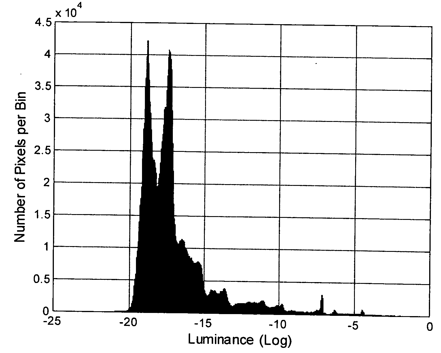
[0008] FIG. 1 shows a histogram.
DETAILED DESCRIPTION OF THE EMBODIMENTS
[0009] The invention will now be described in more detail wherein a method adjusts the exposure of each region based on the overall brightness level of the original HDR image.
[0010] In order to display an HDR image on a LDR display device, a tone mapping method must be employed to map the HDR image, which is usually available as radiance, to 8 bit RGB index numbers. The tone mapping process is not straight forward because it has to simulate the process that happens in the HVS so that the tone mapped LDR image can deceive the HVS into believing it is close enough to the original HDR image. This requires the tone mapping algorithm to be able to maintain both the local contrast and the perceptual brightness.
[0011] The method according to the invention includes a zone-based tone mapping framework which divides the image into regions and then estimates the exposure of each region. The estimation of the exposure, however, maximizes the use of the dynamic range on the tone mapped image, without special consideration to the overall look (brightness) of the tone mapped image compared to the original HDR image.
[0012] The idea behind the method is to obtain the most appropriate exposure for each region with similar illumination. It in fact resonates the concept from photography called zone system and the manual tone mapping methods invented by photographers like Ansel Adams (Adams, A. "The Negative", The Ansel Adams Photography series. Little, Brown and Company. 1981). The disclosed framework has shown advantages in HDR tone mapping.
[0013] Region segmentation is a crucial component throughout the whole method. It seeks to divide the HDR image into different regions where pixels in each of them share the same illumination. One can consider each region has its own "best exposure" value. To accurately segment regions, the correct exposure value is obtained for each region.
[0014] Two region segmentation methods are presented below on the basis of K-means clustering and differential equations, respectively.
[0015] In summary, region segmentation plays a critical role in the tone mapping process. It is usually a rather challenging problem to decide the number of regions and how to segment the HDR image into regions automatically.
[0016] The traditional region segmentation is a very subjective task and it is conducted manually. Well-trained photographers decide how to segment the image into different regions and which zone each region of a photo belongs to with their multiple-years experience and complicated procedure such as using a light meter to record the light condition for each key element in the scene during shooting [Adams, A. "The Print", The Ansel Adams Photography series. Little, Brown and Company. 1981].
[0017] A simple region segmentation method has advantages such as being simple to implement and producing good results for some test images. This method, however, has several drawbacks, such as arbitrarily chosen region position.
[0018] In the framework proposed by Krawczyk [Grzegorz Krawczyk, Karol Myszkowski, Hans-Peter Seidel, "Computational Model of Lightness Perception in High Dynamic Range Imaging", In Proc. of IS&T/SPIE's Human Vision and Electronic Imaging, 2006], given the centroids obtained from K-means clustering, only those with very large number of pixels belonging to them are considered. It is, however, not always desirable in HDR region segmentation since it neglects regions with relatively small number of pixels yet important details, which is usually the case when the dynamic range is very high.
[0019] For segmentation on HDR images, one region can be associated with an approximate luminance range in a scene (i.e. a segment in the histogram of an HDR image, FIG. 1). Hence, in HDR tone reproduction, incorrect region position leads to undesired exposure value for each LDR image. Furthermore, an inappropriate number of regions will either bring up computational complexity when the number is unnecessarily large or result in a region distribution incapable of covering the whole histogram of the HDR image when the number is too small.
[0020] The HDR image segmentation can be a hard or a fuzzy one. In either case, each region is represented by a matrix of the same size as the original HDR image. Each element of the matrix is the probability (weight) of the pixel belonging to this region. If a hard segmentation is applied, one pixel belongs to a single region and thus the weight is either 0 or 1. For the case of fuzzy segmentation, each pixel can spread over several (even all) regions, and consequently the probability can take any value between 0 and 1.
[0021] Anchor point is defined as follows: any pixel in an HDR image is saturated and mapped to one if the luminance of that pixel exceeds the anchor point; otherwise it will be mapped to a value between 0 and 1. Once the anchor point of each region is known, a weight of each pixel for each region can computed. In general, for each region (defined by the corresponding anchor point A.sub.i) in a single exposure image, the closer the pixel intensity is to 0.5 (which corresponds to mid-grey), the larger the weight of that pixel for that region.
[0022] A histogram of an HDR image can span over 10 stops (in photography, stops are a unit used to quantify ratios of light or exposure, with one stop meaning a factor of two), as shown in FIG. 1, while one LDR image can have contrast ratio ranging from 4 to 8 stops. The segmentation methods seek to utilize the information from the image histogram.
1. Region Segmentation Methods
[0023] 1.1. K-Mean Clustering Based Method
[0024] To divide the radiance range properly, the concept of clustering can be utilized, as used for exploratory data analysis. There have been numerous clustering approaches, such as hierarchical clustering, partitional clustering and spectral clustering. Among them, K-means clustering is one of the most popular and widely studied clustering methods for points in Euclidean space. In one dimension, it is a good way to quantize real valued variables into k non-uniform buckets.
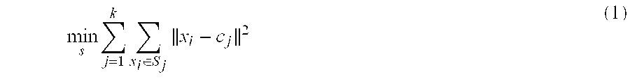
[0025] The K-means formulation assumes that the clusters are defined by the distance of the points to their class centroids only. In other words, given a set of observations (x.sub.1, x.sub.2 . . . , x.sub.n) where each observation x.sub.i is a d-dimensional real vector, the goal of clustering is to find those k mean vectors c.sub.l, . . . , c.sub.k and provide the cluster assignment y.sub.i of each point x.sub.i in the set, such that this set can be partitioned into k partitions (k<n) S={S.sub.1, S.sub.2, . . . , S.sub.k}. The K-means algorithm is based on an interleaving approach where the cluster assignments y.sub.i are established given the centers and the centers are computed given the assignments. The optimization criterion is as follows:
min s j = 1 k x i .di-elect cons. S j x i - c j 2 ( 1 ) ##EQU00001##
where c.sub.j is the centroid of S.sub.j.
[0026] A method utilizes the K-mean clustering to get the anchor points. It can be described as following steps:
[0027] Step 1: First calculate the range of the histogram in logarithm luminance domain with base two and then decide the number of partitions k according to the following equation
k = log 2 ( L max L min ) / .lamda. ( 2 ) ##EQU00002##
where L.sub.max and L.sub.min are the maximum and minimum luminance of the image, respectively. Note here since overlapping between the regions sometimes is desirable, .lamda. is chosen as 4 heuristically.
[0028] Step 2: To obtain the mean value of each region, K-means clustering is applied in log 2 luminance domain. The basic procedure is as follows.
[0029] The observation set (x.sub.1, x.sub.2, . . . , x.sub.n) is the value of log 2 luminance of each pixel. And the centroid of each cluster is denoted as c.sub.l, . . . , c.sub.k.
[0030] 1) Initialize the Clustering.
[0031] There are numerous ways for initialization. Two classical methods are random seed and random partition. In this example k seed points are randomly selected as the initial guess for the centroids in various ways.
[0032] 2) Assign the Data.
[0033] Given the estimated centroids for the current round, the new assignments are computed by the closest center to each point x.sub.i. Assume that c.sub.l, . . . , c.sub.k are given from the previous iteration, then
y i = arg min j x i - c j 2 ( 3 ) ##EQU00003##
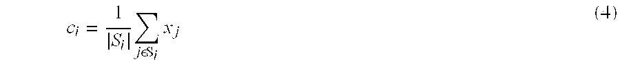
[0034] 3) Update the Centroids.
[0035] Given the updated assignments, the new centers are estimated by taking the mean of each cluster. For any set, one can have
c i = 1 S i j .epsilon.S i x j ( 4 ) ##EQU00004##
[0036] The procedure is conducted in an iterative fashion until the maximum number of iteration step is reached or when the assignments no longer change. Since each step is guaranteed to reduce the optimization energy the process must converge to some local optimum.
[0037] Step 3: Calculate the Anchor Points with the Mean Value Obtained Above.
[0038] Given the centroid values, a half distance between any two adjacent centroids is computed, denoted as l.sub.i(i=1, 2, . . . , k)
l i = { ( c i + 1 - c i ) / 2 i = 1 , 2 , , k - 1 ( l max - c i ) / 2 i = k ( 5 ) ##EQU00005##
[0039] Afterwards, the anchor points are defined as follows
A.sub.i=c.sub.i+min(l.sub.i,.lamda.) i=1, 2, . . . , k (6)
where .lamda. is chosen as 4 empirically.
[0040] Step 4: Once the anchor point of each region is known, the weight of each pixel is computed for each region. In general, for each region (defined by the corresponding anchor point A.sub.i), the closest the value of a pixel in the single exposure image is to 0.5, the larger the weight of that pixel for that region (defined by the corresponding anchor point A.sub.i).
Thus, the weight of pixel at location (i, j) for region n (defined by anchor point A.sub.n) can be computed as below:
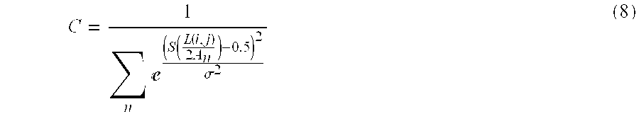
W n ( i , j ) = C ( S ( L ( i , j ) A n ) - 0.5 ) 2 .sigma. 2 ( 7 ) ##EQU00006##
where C is a normalization factor and it is defined as:
C = 1 n ( S ( L ( i , j ) 2 A n ) - 0.5 ) 2 .sigma. 2 ( 8 ) ##EQU00007##
[0041] The above computed weights take values in the range [0,1] and hence define a fuzzy segmentation of the luminance image into N regions. This means each region might contain all the pixels in the image, although only a portion of them might have large weights.
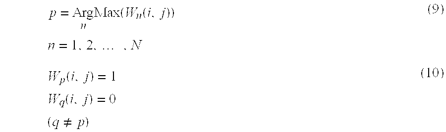
[0042] In another implementation, the weights are binarized (i.e. make them either 0 or 1), resulting in a hard segmentation:
p = Arg n Max ( W n ( i , j ) ) n = 1 , 2 , , N ( 9 ) W p ( i , j ) = 1 W q ( i , j ) = 0 ( q .noteq. p ) ( 10 ) ##EQU00008##
[0043] Note that the anchor points A.sub.n as well as the weights W.sub.n are fixed once the segmentation is done.
[0044] 1.2. Differential Equations Based Method
[0045] In the following, an alternate embodiment method to use PDEs for region segmentation will be described as follows.
[0046] Step 1: Design the Cost Function (Energy Function)
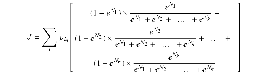
[0047] The goal is to obtain the best exposure for each region. To accomplish this, an energy function is designed as
J = i p L i [ ( 1 - N 1 ) .times. N 1 N 1 + N 2 + + N k + ( 1 - N 2 ) .times. N 2 N 1 + N 2 + + N k + + ( 1 - N k ) .times. N k N 1 + N 2 + + N k ] ( 11 ) N j = - [ S ( L 1 A j ) - 0.5 ] 2 .sigma. 2 ( j = 1 , 2 , , k ) ( 12 ) ##EQU00009##
where i is the index of bins in the histogram, L.sub.i is the corresponding luminance value, P.sub.L is the probability of L.sub.i, {A.sub.j} are the anchor points sought, .sigma. is a constant, which equals to 0.2 in the disclosed implementation, and S(.cndot.) is the saturation function, which is defined as follows:
S ( x ) = { 1 x > 1 x 1 / .gamma. otherwise ( 13 ) ##EQU00010##
where .gamma. optimally takes values in the range [2.2,2.4].
[0048] In Eq. (12), Gaussian curve e.sup.(.cndot.) serves as a measurement for exposure. The closer the luminance is to 0.5, the better the exposure is.
[0049] Step 2: Solve the Optimization Problem
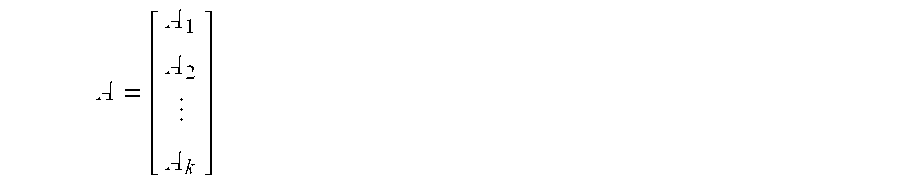
[0050] Using a chain rule, differentiation of energy function J with respect to anchor point set
A = [ A 1 A 2 A k ] ##EQU00011##
can be obtained, noted as
J A . ##EQU00012##
In order to minimize the energy function, can a gradient descent method can be utilized, i.e.,
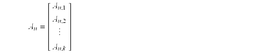
A.sub.n+1=A.sub.n-.gamma..gradient.J(A.sub.A) (14)
where
A n = [ A n , 1 A n , 2 A n , k ] ##EQU00013##
and .gamma. is the step-size parameter. Eq. (14) is iterated until the maximum number of iteration step is reached or the prescribed accuracy is met, i.e., .parallel.A.sub.n+1-A.sub.n.parallel..ltoreq..epsilon., where .epsilon. is a given small positive value.
J A ##EQU00014##
is used in an iterative procedure, which at each step seeks to decrease the error. Upon convergence, the anchor points are local optimum of the energy function.
[0051] Step 3: Once the anchor point of each region is known, compute the weight of each pixel for each region as described above.
[0052] The foregoing illustrates some of the possibilities for practicing the invention. Many other embodiments are possible within the scope and spirit of the invention. For example, alternatively in Section 1.2 step 2, there other methods than gradient descent can be used to solve the optimization problem. It is, therefore, intended that the foregoing description be regarded as illustrative rather than limiting, and that the scope of the invention is given by the appended claims together with their full range of equivalents.
* * * * *
D00000
D00001


XML
uspto.report is an independent third-party trademark research tool that is not affiliated, endorsed, or sponsored by the United States Patent and Trademark Office (USPTO) or any other governmental organization. The information provided by uspto.report is based on publicly available data at the time of writing and is intended for informational purposes only.
While we strive to provide accurate and up-to-date information, we do not guarantee the accuracy, completeness, reliability, or suitability of the information displayed on this site. The use of this site is at your own risk. Any reliance you place on such information is therefore strictly at your own risk.
All official trademark data, including owner information, should be verified by visiting the official USPTO website at www.uspto.gov. This site is not intended to replace professional legal advice and should not be used as a substitute for consulting with a legal professional who is knowledgeable about trademark law.