Method and apparatus for adaptive exposure bracketing, segmentation and scene organization
El Dokor , et al.
U.S. patent number 10,721,448 [Application Number 13/831,638] was granted by the patent office on 2020-07-21 for method and apparatus for adaptive exposure bracketing, segmentation and scene organization. This patent grant is currently assigned to Edge 3 Technologies, Inc.. The grantee listed for this patent is Edge 3 Technologies, Inc.. Invention is credited to Jordan Cluster, Tarek El Dokor, Joshua King.


View All Diagrams
| United States Patent | 10,721,448 |
| El Dokor , et al. | July 21, 2020 |
Method and apparatus for adaptive exposure bracketing, segmentation and scene organization
Abstract
A method, system and computer program are provided that present a real-time approach to Chromaticity maximization to be used in image segmentation. The ambient illuminant in a scene may be first approximated. The input image may then be preprocessed to remove the impact of the illuminant, and approximate an ambient white light source instead. The resultant image is then choma-maximized. The result is an adaptive Chromaticity maximization algorithm capable of adapting to a wide dynamic range of illuminations. A segmentation algorithm is put in place as well that takes advantage of such an approach. This approach also has applications in HDR photography and real-time HDR video.
| Inventors: | El Dokor; Tarek (Phoenix, AZ), Cluster; Jordan (Tempe, AZ), King; Joshua (Mesa, AZ) | ||||||||||
|---|---|---|---|---|---|---|---|---|---|---|---|
| Applicant: |
|
||||||||||
| Assignee: | Edge 3 Technologies, Inc.
(Phoenix, AZ) |
||||||||||
| Family ID: | 51525596 | ||||||||||
| Appl. No.: | 13/831,638 | ||||||||||
| Filed: | March 15, 2013 |
Prior Publication Data
| Document Identifier | Publication Date | |
|---|---|---|
| US 20140267612 A1 | Sep 18, 2014 | |
| Current U.S. Class: | 1/1 |
| Current CPC Class: | G06K 9/4661 (20130101); H04N 9/735 (20130101); H04N 5/2356 (20130101) |
| Current International Class: | H04N 9/73 (20060101); G06K 9/46 (20060101); H04N 5/235 (20060101) |
References Cited [Referenced By]
U.S. Patent Documents
| 5454043 | September 1995 | Freeman |
| 5504524 | April 1996 | Lu et al. |
| 5544050 | August 1996 | Abe et al. |
| 5581276 | December 1996 | Cipolla et al. |
| 5594469 | January 1997 | Freeman et al. |
| 5699441 | December 1997 | Sagawa et al. |
| 5767842 | June 1998 | Korth |
| 5887069 | March 1999 | Sakou et al. |
| 5990865 | November 1999 | Gard |
| 6002808 | December 1999 | Freeman |
| 6072494 | June 2000 | Nguyen |
| 6075895 | June 2000 | Qiao et al. |
| 6115482 | September 2000 | Sears et al. |
| 6128003 | October 2000 | Smith et al. |
| 6141434 | October 2000 | Christian et al. |
| 6147678 | November 2000 | Kumar et al. |
| 6181343 | January 2001 | Lyons |
| 6195104 | February 2001 | Lyons |
| 6204852 | March 2001 | Kumar et al. |
| 6215890 | April 2001 | Matsuo et al. |
| 6222465 | April 2001 | Kumar et al. |
| 6240197 | May 2001 | Christian et al. |
| 6240198 | May 2001 | Rehg et al. |
| 6252598 | June 2001 | Segen |
| 6256033 | July 2001 | Nguyen |
| 6256400 | July 2001 | Takata et al. |
| 6269172 | July 2001 | Rehg et al. |
| 6323942 | November 2001 | Bamji |
| 6324453 | November 2001 | Breed et al. |
| 6360003 | March 2002 | Doi et al. |
| 6363160 | March 2002 | Bradski et al. |
| 6377238 | April 2002 | McPheters |
| 6389182 | May 2002 | Ihara et al. |
| 6394557 | May 2002 | Bradski |
| 6400830 | June 2002 | Christian et al. |
| 6434255 | August 2002 | Harakawa |
| 6442465 | August 2002 | Breed et al. |
| 6456728 | September 2002 | Doi et al. |
| 6478432 | November 2002 | Dyner |
| 6509707 | January 2003 | Yamashita et al. |
| 6512838 | January 2003 | Rafii et al. |
| 6526156 | February 2003 | Black et al. |
| 6553296 | April 2003 | Breed et al. |
| 6556708 | April 2003 | Christian et al. |
| 6571193 | May 2003 | Unuma et al. |
| 6590605 | July 2003 | Eichenlaub |
| 6600475 | July 2003 | Gutta et al. |
| 6608910 | August 2003 | Srinivasa et al. |
| 6614422 | September 2003 | Rafii et al. |
| 6624833 | September 2003 | Kumar et al. |
| 6674877 | January 2004 | Jojic et al. |
| 6674895 | January 2004 | Rafii et al. |
| 6678425 | January 2004 | Flores et al. |
| 6681031 | January 2004 | Cohen et al. |
| 6683968 | January 2004 | Pavlovic et al. |
| 6757571 | June 2004 | Toyama |
| 6766036 | July 2004 | Pryor |
| 6768486 | July 2004 | Szabo et al. |
| 6788809 | September 2004 | Grzeszczuk et al. |
| 6795567 | September 2004 | Cham et al. |
| 6801637 | October 2004 | Voronka et al. |
| 6804396 | October 2004 | Higaki et al. |
| 6829730 | December 2004 | Nadeau-Dostie et al. |
| 6857746 | February 2005 | Dyner |
| 6901561 | May 2005 | Kirkpatrick et al. |
| 6937742 | August 2005 | Roberts et al. |
| 6940646 | September 2005 | Taniguchi et al. |
| 6944315 | September 2005 | Zipperer et al. |
| 6950534 | September 2005 | Cohen et al. |
| 6993462 | January 2006 | Pavlovic et al. |
| 7039676 | May 2006 | Day et al. |
| 7046232 | May 2006 | Inagaki et al. |
| 7050606 | May 2006 | Paul et al. |
| 7050624 | May 2006 | Dialameh et al. |
| 7058204 | June 2006 | Hildreth et al. |
| 7065230 | June 2006 | Yuasa et al. |
| 7068842 | June 2006 | Liang et al. |
| 7095401 | August 2006 | Liu et al. |
| 7102615 | September 2006 | Marks |
| 7129927 | October 2006 | Mattson |
| 7170492 | January 2007 | Bell |
| 7190811 | March 2007 | Ivanov |
| 7203340 | April 2007 | Gorodnichy |
| 7212663 | May 2007 | Tomasi |
| 7221779 | May 2007 | Kawakami et al. |
| 7224830 | May 2007 | Nefian et al. |
| 7224851 | May 2007 | Kinjo |
| 7233320 | June 2007 | Lapstun et al. |
| 7236611 | June 2007 | Roberts et al. |
| 7239718 | July 2007 | Park et al. |
| 7257237 | August 2007 | Luck et al. |
| 7274800 | September 2007 | Nefian et al. |
| 7274803 | September 2007 | Sharma et al. |
| 7289645 | October 2007 | Yamamoto et al. |
| 7295709 | November 2007 | Cootes et al. |
| 7296007 | November 2007 | Funge et al. |
| 7308112 | November 2007 | Fujimura et al. |
| 7340077 | March 2008 | Gokturk et al. |
| 7340078 | March 2008 | Shikano et al. |
| 7342485 | March 2008 | Joehl et al. |
| 7346192 | March 2008 | Yuasa et al. |
| 7348963 | March 2008 | Bell |
| 7359529 | April 2008 | Lee |
| 7372977 | May 2008 | Fujimura et al. |
| 7379563 | May 2008 | Shamaie |
| 7391409 | June 2008 | Zalewski et al. |
| 7394346 | July 2008 | Bodin |
| 7412077 | August 2008 | Li et al. |
| 7415126 | August 2008 | Breed et al. |
| 7415212 | August 2008 | Matsushita et al. |
| 7421093 | September 2008 | Hildreth et al. |
| 7423540 | September 2008 | Kisacanin |
| 7444001 | October 2008 | Roberts et al. |
| 7450736 | November 2008 | Yang et al. |
| 7460690 | December 2008 | Cohen et al. |
| 7477758 | January 2009 | Piirainen et al. |
| 7489308 | February 2009 | Blake et al. |
| 7489806 | February 2009 | Mohri et al. |
| 7499569 | March 2009 | Sato et al. |
| 7512262 | March 2009 | Criminisi et al. |
| 7519223 | April 2009 | Dehlin et al. |
| 7519537 | April 2009 | Rosenberg |
| 7574020 | August 2009 | Shamaie |
| 7590262 | September 2009 | Fujimura et al. |
| 7593552 | September 2009 | Higaki et al. |
| 7598942 | October 2009 | Underkoffler et al. |
| 7599547 | October 2009 | Sun et al. |
| 7606411 | October 2009 | Venetsky et al. |
| 7612813 | November 2009 | Hunter |
| 7614019 | November 2009 | Rimas Ribikauskas et al. |
| 7620316 | November 2009 | Boillot |
| 7646372 | January 2010 | Marks et al. |
| 7660437 | February 2010 | Breed |
| 7665041 | February 2010 | Wilson et al. |
| 7676062 | March 2010 | Breed et al. |
| 7720282 | May 2010 | Blake et al. |
| 7721207 | May 2010 | Nilsson |
| 7804998 | September 2010 | Mundermann Lars et al. |
| 2001/0001182 | May 2001 | Ito et al. |
| 2001/0030642 | October 2001 | Sullivan et al. |
| 2002/0041327 | April 2002 | Hildreth et al. |
| 2002/0064382 | May 2002 | Hildreth et al. |
| 2002/0090133 | July 2002 | Kim et al. |
| 2002/0140633 | October 2002 | Rafii et al. |
| 2002/0176010 | November 2002 | Wallach et al. |
| 2004/0183775 | September 2004 | Bell |
| 2005/0002074 | January 2005 | McPheters et al. |
| 2005/0083314 | April 2005 | Shalit et al. |
| 2005/0105775 | May 2005 | Luo et al. |
| 2005/0190443 | September 2005 | Nam et al. |
| 2005/0286756 | December 2005 | Hong et al. |
| 2006/0093186 | May 2006 | Ivanov |
| 2006/0101354 | May 2006 | Hashimoto et al. |
| 2006/0136846 | June 2006 | Im et al. |
| 2006/0139314 | June 2006 | Bell |
| 2006/0221072 | October 2006 | Se et al. |
| 2007/0055427 | March 2007 | Sun et al. |
| 2007/0113207 | May 2007 | Gritton |
| 2007/0132721 | June 2007 | Glomski et al. |
| 2007/0195997 | August 2007 | Paul et al. |
| 2007/0211165 | September 2007 | Yaguchi |
| 2007/0263932 | November 2007 | Bernardin et al. |
| 2007/0280505 | December 2007 | Breed |
| 2008/0002878 | January 2008 | Meiyappan et al. |
| 2008/0005703 | January 2008 | Radivojevic et al. |
| 2008/0013793 | January 2008 | Hillis et al. |
| 2008/0037875 | February 2008 | Kim et al. |
| 2008/0052643 | February 2008 | Ike et al. |
| 2008/0059578 | March 2008 | Albertson et al. |
| 2008/0065291 | March 2008 | Breed |
| 2008/0069415 | March 2008 | Schildkraut et al. |
| 2008/0069437 | March 2008 | Baker |
| 2008/0104547 | May 2008 | Morita et al. |
| 2008/0107303 | May 2008 | Kim et al. |
| 2008/0120577 | May 2008 | Ma et al. |
| 2008/0178126 | July 2008 | Beeck et al. |
| 2008/0181459 | July 2008 | Martin et al. |
| 2008/0219501 | September 2008 | Matsumoto |
| 2008/0219502 | September 2008 | Shamaie |
| 2008/0225041 | September 2008 | El Dokor et al. |
| 2008/0229255 | September 2008 | Linjama et al. |
| 2008/0240502 | October 2008 | Freedman et al. |
| 2008/0244465 | October 2008 | Kongqiao et al. |
| 2008/0244468 | October 2008 | Nishihara et al. |
| 2008/0267449 | October 2008 | Dumas et al. |
| 2008/0282202 | November 2008 | Sunday |
| 2009/0006292 | January 2009 | Block |
| 2009/0027337 | January 2009 | Hildreth |
| 2009/0037849 | February 2009 | Immonen et al. |
| 2009/0040215 | February 2009 | Afzulpurkar et al. |
| 2009/0060268 | March 2009 | Roberts et al. |
| 2009/0074248 | March 2009 | Cohen et al. |
| 2009/0077504 | March 2009 | Bell et al. |
| 2009/0079813 | March 2009 | Hildreth |
| 2009/0080526 | March 2009 | Vasireddy et al. |
| 2009/0085864 | April 2009 | Kutliroff et al. |
| 2009/0102788 | April 2009 | Nishida et al. |
| 2009/0102800 | April 2009 | Keenan |
| 2009/0103780 | April 2009 | Nishihara et al. |
| 2009/0108649 | April 2009 | Kneller et al. |
| 2009/0109036 | April 2009 | Schalla et al. |
| 2009/0110292 | April 2009 | Fujimura et al. |
| 2009/0115721 | May 2009 | Aull et al. |
| 2009/0116742 | May 2009 | Nishihara |
| 2009/0116749 | May 2009 | Cristinacce et al. |
| 2009/0150160 | June 2009 | Mozer |
| 2009/0153366 | June 2009 | Im et al. |
| 2009/0153655 | June 2009 | Ike et al. |
| 2009/0180668 | July 2009 | Jones et al. |
| 2009/0183125 | July 2009 | Magal et al. |
| 2009/0183193 | July 2009 | Miller, IV |
| 2009/0189858 | July 2009 | Lev et al. |
| 2009/0208057 | August 2009 | Wilson et al. |
| 2009/0222149 | September 2009 | Murray et al. |
| 2009/0228841 | September 2009 | Hildreth |
| 2009/0231278 | September 2009 | St Hilaire et al. |
| 2009/0244309 | October 2009 | Maison et al. |
| 2009/0249258 | October 2009 | Tang |
| 2009/0262986 | October 2009 | Cartey et al. |
| 2009/0268945 | October 2009 | Wilson et al. |
| 2009/0273563 | November 2009 | Pryor |
| 2009/0273574 | November 2009 | Pryor |
| 2009/0273575 | November 2009 | Pryor |
| 2009/0278915 | November 2009 | Kramer et al. |
| 2009/0295738 | December 2009 | Chiang |
| 2009/0296991 | December 2009 | Anzola |
| 2009/0315740 | December 2009 | Hildreth et al. |
| 2009/0316952 | December 2009 | Ferren et al. |
Other References
|
Freeman, W. T. et al., "The Design and Use of Steerable Filters", IEEE Transactions of Pattern Analysis and Machine Intelligence V. 13, (Sep. 1991),891-906. cited by applicant . Simoncelli, E.P. et al., "Shiftable Multi-scale Transforms", IEEE Transactions on Information Theory V. 38, (Mar. 1992),587-607. cited by applicant . Simoncelli, E.P. et al., "The Steerable Pyramid: A Flexible Architecture for Multi-Scale Derivative Computation", Proceedings of ICIP-95 V. 3, (Oct. 1995),444-447. cited by applicant . Chen, J et al., "Adaptive Perceptual Color-Texture Image Segmentation", IEEE Transactions on Image Processing, v. 14, No. 10, (Oct. 2005),1524-1536 (2004 revised draft). cited by applicant . Halfhill, Tom R., "Parallel Processing with CUDA", Microprocessor Report, Available at http://www.nvidia.com/docs/IO/55972/220401_Reprint.pdf,(Jan. 28, 2008). cited by applicant . Farber, Rob "CUDA, Supercomputing for the Masses: Part 4, The CUDA Memory Model", Under the High Performance Computing section of the Dr. Dobbs website, p. 3 available at http://www.ddj.com/hpc-high-performance-computing/208401741, 3. cited by applicant . Rajko, S et al., "HMM Parameter Reduction for Practice Gesture Recognition", Proceedings of the International Conference on Automatic Gesture Recognition, (Sep. 2008). cited by applicant . Hinton, Geoffrey et al., "A Fast Learning Algorithm for Deep Belief Nets", Neural Computation, V. 18, 1527-1554. cited by applicant . Susskind, Joshua M., et al., "Generating Facial Expressions with Deep Belief Nets", Department of Psychology, Univ. of Toronto I-Tech Education and Publishing, (2008),421-440. cited by applicant . Bleyer, Michael et al., "Surface Stereo with Soft Segmentation.", Computer Vision and Pattern Recognition. IEEE, 2010, (2010). cited by applicant . Chen, Junqing et al., "Adaptive perceptual color-texture image segmentation.",The International Society for Optical Engineering, SPIE Newsroom, (2006),1-2. cited by applicant . Forsyth, David A., et al., "Stereopsis", In Computer Vision a Modern Approach Prentice Hall, 2003, (2003). cited by applicant . Harris, Mark et al., "Parallel Prefix Sum (Scan) with CUDA", vol. 39 in GPU Gems 3, edited by Hubert Nguyen, (2007). cited by applicant . Hirschmuller, Heiko "Stereo Vision in Structured Environments by Consistent Semi-Global Matching", Computer Vision and Pattern Recognition, CVPR 06, (2006),2386-2393. cited by applicant . Ivekovic, Spela et al., "Dense Wide-baseline Disparities from Conventional Stereo for Immersive Videoconferencing", ICPR. 2004, (2004),921-924. cited by applicant . Kaldewey, Tim et al., "Parallel Search on Video Cards.", First USENIX Workshop on Hot Topics in Parallelism(HotPar '09), (2009). cited by applicant . Kirk, David et al., "Programming Massively Parallel Processors a Hands-on Approach", Elsevier, 2010, (2010). cited by applicant . Klaus, Andreas et al., "Segment-Based Stereo Matching Using Belief Propagation and a Self-Adapting Dissimilarity Measure", Proceedings of ICPR 2006. IEEE, 2006, (2006),15-18. cited by applicant . Kolmogorov, Vladimir et al., "Computing Visual Correspondence with Occlusions via Graph Cuts", International Conference on Computer Vision. 2001., (2001). cited by applicant . Kolmogorov, Vladimir et al., "Generalized Multi-camera Scene Reconstruction Using Graph Cuts.", Proceedings for the International Workshop on Energy Minimization Methods in Computer Vision and Pattern Recognition. 2003., (2003). cited by applicant . Kuhn, Michael et al., "Efficient ASIC Implementation of a Real-Time Depth Mapping Stereo Vision System", Proceedings of 2009 IEEE International Conference on Acoustics, Speech and Signal Processing. Taipei, Taiwan: IEEE, 2009., (2009). cited by applicant . Li, Shigang "Binocular Spherical Stereo", IEEE Transactions on Intelligent Transportation Systems(IEEE) 9, No. 4 (Dec. 2008), (Dec. 2008),589-600. cited by applicant . Marsalek, M et al., "Semantic hierarchies for visual object recognition", Proceedings of IEEE Conference on Computer Vision and Pattern Recognition, 2007. CVPR '07. MN: IEEE, 2007, (2007),1-7. cited by applicant . Metzger, Wolfgang "Laws of Seeing", MIT Press, 2006, (2006). cited by applicant . Min, Dongbo et al., "Cost Aggregation and Occlusion Handling With WLS in Stereo Matching", Edited by IEEE. IEEE Transactions on Image Processing 17(2008), (2008),1431-1442. cited by applicant . "NVIDIA: CUDA compute unified device architecture, prog. guide, version 1.1", NVIDIA, (2007). cited by applicant . Remondino, Fabio et al., "Turning Images into 3-D Models", IEEE Signal Processing Magazine, (2008). cited by applicant . Richardson, Ian E., "H.264/MPEG-4 Part 10 White Paper", White Paper/www.vcodex.com, (2003). cited by applicant . Sengupta, Shubhabrata "Scan Primitives for GPU Computing", Proceedings of the 2007 Graphics Hardware Conference. San Diego, CA, 2007, (2007),97-106. cited by applicant . Sintron, Eric et al., "Fast Parallel GPU-Sorting Using a Hybrid Algorithm", Journal of Parallel and Distributed Computing (Elsevier) 68, No. 10, (Oct. 2008),1381-1388. cited by applicant . Wang, Zeng-Fu et al., "A Region Based Stereo Matching Algorithm Using Cooperative Optimization", CVPR (2008). cited by applicant . Wei, Zheng et al., "Optimization of Linked List Prefix Computations on Multithreaded GPUs Using CUDA", 2010 IEEE International Symposium on Parallel & Distributed Processing(IPDPS). Atlanta, (2010). cited by applicant . Wiegand, Thomas et al., "Overview of the H.264/AVC Video Coding Standard", IEEE Transactions on Circuits and Systems for Video Technology 13 , No. 7 (Jul. 2003),560-576. cited by applicant . Woodford, O.J. et al., "Global Stereo Reconstruction under Second Order Smoothness Priors", IEEE Transactions on Pattern Analysis and Machine Intelligence(IEEE) 31, No. 12, (2009),2115-2128. cited by applicant . Yang, Qingxiong et al., "Stereo Matching with Color-Weighted Correlation, Hierarchical Belief Propagation, and Occlusion Handling", IEEE Transactions on Pattern Analysis and Machine Intelligence(IEEE) 31, No. 3, (Mar. 2009),492-504. cited by applicant . Zinner, Christian et al., "An Optimized Software-Based Implementation of a Census-Based Stereo Matching Algorithm", Lecture Notes in Computer Science(SpringerLink) 5358, (2008),216-227. cited by applicant . "PCT Search report", PCT/US2010/035717, (dated Sep. 1, 2010),1-29. cited by applicant . "PCT Written opinion", PCT/US2010/035717, (dated Dec. 1, 2011),1-9. cited by applicant . "PCT Search report", PCT/US2011/49043, (dated Mar. 21, 2012), 1-4. cited by applicant . "PCT Written opinion", PCT/US2011/49043, (dated Mar. 21, 2012), 1-4. cited by applicant . "PCT Search report", PCT/US2011/049808, (dated Jan. 12, 2012), 1-2. cited by applicant . "PCT Written opinion", PCT/US2011/049808, (dated Jan. 12, 2012), 1-5. cited by applicant . "Non-Final Office Action", U.S. Appl. No. 12/784,123, (dated Oct. 2, 2012), 1-20. cited by applicant . "Non-Final Office Action", U.S. Appl. No. 12/784,022, (dated Jul. 16, 2012), 1-14. cited by applicant . Tieleman, T et al., "Using Fast weights to improve persistent contrastive divergence", 26th International Conference on Machine Learning New York, NY ACM, (2009),1033-1040. cited by applicant . Sutskever, I et al., "The recurrent temporal restricted boltzmann machine", NIPS, MIT Press, (2008),1601-1608. cited by applicant . Parzen, E "On the estimation of a probability density function and the mode", Annals of Math. Stats., 33, (1962),1065-1076. cited by applicant . Hopfield, J.J. "Neural networks and physical systems with emergent collective computational abilities", National Academy of Sciences, 79, (1982),2554-2558. cited by applicant . Culibrk, D et al., "Neural network approach to background modeling for video object segmentation", IEEE Transactions on Neural Networks, 18, (2007),1614-1627. cited by applicant . Benggio, Y et al., "Curriculum learning", ICML 09 Proceedings of the 26th Annual International Conference on Machine Learning, New York, NY: ACM, (2009). cited by applicant . Benggio, Y et al., "Scaling learning algorithms towards AI. In L. a Bottou", Large Scale Kernel Machines, MIT Press,(2007). cited by applicant . Battiato, S et al., "Exposure correction for imaging devices: An overview", In R. Lukac (Ed.), Single Sensor Imaging Methods and Applications for Digital Cameras, CRC Press,(2009),323-350. cited by applicant . U.S. Appl. No. 12/028,704, filed Feb. 2, 2008, Method and System for Vision-Based Interaction in a Virtual Environment. cited by applicant . U.S. Appl. No. 13/405,319, filed Feb. 26, 2012, Method and System for Vision-Based Interaction in a Virtual Environment. cited by applicant . U.S. Appl. No. 13/411,657, filed Mar. 5, 2012, Method and System for Vision-Based Interaction in a Virtual Environment. cited by applicant . U.S. Appl. No. 13/429,437, filed Mar. 25, 2012, Method and System for Vision-Based Interaction in a Virtual Environment. cited by applicant . U.S. Appl. No. 13/562,351, filed Jul. 31, 2012, Method and System for Tracking of a Subject. cited by applicant . U.S. Appl. No. 13/596,093, filed Aug. 28, 2012 Method and Apparatus for Three Dimensional Interaction of a Subject. cited by applicant . U.S. Appl. No. 11/567,888, filed Dec. 7, 2006, Three-Dimensional Virtual-Touch Human-Machine Interface System and Method Therefor. cited by applicant . U.S. Appl. No. 13/572,721, filed Aug. 13, 2012, Method and System for Three-Dimensional Virtual-Touch Interface. cited by applicant . U.S. Appl. No. 12/784,123, filed Mar. 20, 2010, Gesture Recognition Systems and Related Methods. cited by applicant . U.S. Appl. No. 12/784,022, filed May 20, 2010, Systems and Related Methods for Three Dimensional Gesture Recognition in Vehicles. cited by applicant . U.S. Appl. No. 13/025,038, filed Feb. 10, 2011, Method and Apparatus for Performing Segmentation of an Image. cited by applicant . U.S. Appl. No. 13/025,055, filed Feb. 10, 2011, Method and Apparatus for Disparity Computation in Stereo Images. cited by applicant . U.S. Appl. No. 13/025,070, filed Feb. 10, 2011, Method and Apparatus for Determining Disparity of Texture. cited by applicant . U.S. Appl. No. 13/221,903, filed Aug. 31, 2011, Method and Apparatus for Confusion Learning. cited by applicant . U.S. Appl. No. 13/189,517, filed Jul. 24, 2011, Near-Touch Interaction with a Stereo Camera Grid and Structured. cited by applicant . U.S. Appl. No. 13/297,029, filed Nov. 15, 2011, Method and Apparatus for Fast Computational Stereo. cited by applicant . U.S. Appl. No. 13/297,144, filed Nov. 15, 2011, Method and Apparatus for Fast Computational Stereo. cited by applicant . U.S. Appl. No. 13/294,481, filed Nov. 11, 2011, Method and Apparatus for Enhanced Stereo Vision. cited by applicant . U.S. Appl. No. 13/316,606, filed Dec. 12, 2011, Method and Apparatus for Enhanced Stereo Vision. cited by applicant. |
Primary Examiner: Ren; Zhubing
Attorney, Agent or Firm: Kessler; Gordon
Claims
What is claimed:
1. A method for imaging a scene comprising the steps of: determining a camera response function based upon one or more images captured with a camera; synthetically creating profiles of one or more pixels of the one or more images at different exposures; determining an exposure of the one or more pixels in one or more of the one or more images resulting in a maximized chroma in accordance with at least the determined camera response function and one or more perceptual parameters resulting in color consistency; imaging the scene at the exposure resulting in the maximized chroma; and determining a hue associated with the one or more pixels at the exposure resulting in the maximized chroma.
2. The method of claim 1, where in the step of maximizing chroma in an image further comprises the step of employing a set of rolling exposure images to track and compute a max chromaticity.
3. The method of claim 1, wherein the maximizing of chroma maintains color consistency between images.
4. The method of claim 1, further comprising the step of defining color consistency as a hue that is associated with max chromaticity.
5. A method for imaging a scene comprising the steps of: determining a camera response function based upon one or more images captured with a camera; segmenting one or more regions of interest within the one or more captured images; synthetically creating profiles of one or more pixels of the one or more images at different exposures; determining an exposure of the one or more pixels in the one or more images resulting in maximized chroma in each of the one or more regions of interest in accordance with the determined camera response function; imaging the scene at the exposure resulting in the maximized chroma for one or more of the regions of interest; and determining a hue associated with the one or more pixels at the exposure resulting in the maximized chroma.
6. The method of claim 5, further comprising the step of using an ambient illuminant approximator to minimize one or more effects of one or more light sources on the imaging of the scene.
7. The method of claim 6, further comprising the step of tracking color/hue consistency by modeling perceptual elements through the combination of illuminant approximation as well as Chromaticity maximization.
8. The method of claim 5, further comprising the step of segmenting the image based on combining simulated/estimated exposure settings and color/texture/motion features.
9. The method of claim 5, further comprising the step of creating a depth map based on segmentation, combining simulated exposure settings with features of color, texture and motion.
10. A method for imaging a scene comprising the steps of: determining a camera response function based upon one or more images captured with a camera; segmenting one or more regions of interest within the one or more captured images; synthetically creating profiles of one or more pixels of the one or more images comprising the one or more regions of interest at different exposures; determining an exposure of the one or more pixels in the one or more images resulting in maximized chroma in each of the one or more regions of interest in accordance with the determined camera response function; imaging the scene at each exposure resulting in a maximized chroma for each of the one or more of the regions of interest; and generating a composite depth map employing the images generated for each region of interest imaged at the exposure setting resulting in the maximized chroma for that region of interest.
11. The method of claim 10, further comprising the step of using an ambient illuminant approximator to minimize one or more effects of one or more light sources on the imaging of the scene.
12. The method of claim 11, further comprising the step of tracking color/hue consistency by modeling perceptual elements through the combination of illuminant approximation as well as Chromaticity maximization.
13. The method of claim 10, wherein the step of segmenting the image is based on combining simulated/estimated exposure settings and color/texture/motion features.
14. The method of claim 10, wherein the depth map is further generated based on segmentation, combining simulated exposure settings with features of color, texture and motion.
Description
BACKGROUND
Many approaches exist that enable high-quality imaging systems with good image capture quality. These systems, however, fail to provide a complete solution imaging system that includes a given capture system and an associated quality rendering system that can extract the best color settings associated with a given scene.
SUMMARY
Color Constancy in the Human Visual System (HVS) and Illuminant Approximation
Color constancy has been described in Chakrabarti, A., Hirakawa, K., & Zickler, T. (2011), Color Constancy with Spatio-Spectral Statistics. IEEE Transactions on Pattern Analysis and Machine Intelligence, and refers to a property of color descriptors allowing for inference of appropriate colors in spite of changes in lighting. This is therefore a perceptual notion that colors and their perception fundamentally don't change as images change in a scene during subjective testing. As such, colors of various objects are usually perceived uniformly by the Human Visual System in spite of the fact that such objects may change colors as they are being observed, or as they undergo different ambient lighting conditions from different illuminants. Stockman, A., & Brainard, D. (2010). Color vision mechanisms. OSA Handbook of Optics (3rd edition, M. Bass, ed), 11.1-11.104. hence, a very powerful quality of biological vision involves maintaining a robust estimate of the color of objects even as such objects change their perceived color values. This perceptual quality is very powerful and has been the focus of much research on how to emulate color constancy.
Described aptly in (Stockman & Brainard, 2010), "When presented in the same context under photopic conditions, pairs of lights that produce the same excitations in the long-, middle-, and short-wavelength-sensitive (L-, M-, and S-) cones match each other exactly in appearance. Moreover, this match survives changes in context and changes in adaptation, provided that the changes are applied equally to both lights." Biological color constancy, however, has its limits and typically falls short under various conditions. As a fun example, optical illusions are presented in (Lotto's Illusion), where perceptions of different illumination levels, colors, and light sources are presented as examples. As illuminant changes happen drastically in the field-of-view, humans are more likely to confuse color quality. Estimating an illuminant is a good starting point, but compensating for the illuminant is a problem in itself, and has been the subject of much research, see Barnard, K., Cardei, V., & Funt, B. (2002). A comparison of computational color constancy algorithms--Part I: Methodology and experiments with synthesized data. IEEE Trans. Image Processing, 11 (9), 972-984, and Gijsenij, A., Gevers, T., & Weijer, J. (2011). Computational Color Constancy: Survey and Experiments. IEEE Trans. Image Processing, 20 (9), 2475-2489.as example approaches to computing illuminant estimators. Biological vision, while powerful, isn't perfect and can be fooled and confused by a variety of circumstances: it is relatively easy to fool people's visual capacities as well as other animals' by camouflaging colors, and by changing the first and second-order statistics of different objects.
Additionally, estimating the illuminant is an inherently underdetermined problem, i.e., with significantly more scene parameters than there are degrees of freedom in the data. Estimating the illuminant is, hence, an inherently nonlinear problem, with many degrees of freedom. It is therefore important to make some simplifying assumptions before proceeding:
1) The notion of color constancy in the HVS has its limitations and may not be very appropriate to applications where changes in lighting occur rapidly and frequently, such circumstances being very different than what the HVS or even biological vision may be used to.
2) Maintaining a notion of color constancy is less important than maintaining a sense of color consistency. At very high frame rates, with lighting changes occurring suddenly and abruptly, it becomes essential to maintain a notion of color consistency across frames, while not necessarily maintaining color constancy across the entire dataset, potentially comprised of millions of frames.
3) Cameras are not analogous to biological eyes. Cameras may over-expose, under-expose, or use a series of rolling exposures in ways that biological vision is not capable of. Moreover, cameras may be underexposed completely, such that only very little light is incident onto the sensors, and then having depth perception accomplished for whatever little information is present, or having the cameras significantly overexposed, such that significantly darker regions are adequately exposed. While the HVS may use autofocus, vary the aperture, and adapt to changing lighting, the speed with which it does so may hinder high-end machine vision applications. It is important in accordance with one or more embodiments of the invention to be able to preferably vary camera settings at speeds that are significantly greater than possible by the HVS.
4) There is a need to synthetically predict/compute images at different exposures in real-time and at a very high frame rates, given a set of observations. In accordance with this approach presented in accordance with one or more embodiments of the present invention, the entire relevance of the HVS becomes marginalized, relatively to computational models of scene analysis that can extra critical information about the response of the cameras to different illuminants. Again, this is a departure from the usual HVS-inspired approaches.
Therefore, in accordance with one or more embodiments of the present invention, an overview of illuminant estimation, and how such illuminant estimation is applicable to modifying a scene's trichromatic feature set, adapting and compensating for such illuminants will be provided. Various embodiments of the present invention are provided, based on the notion of chromaticity maximization and hue value consistency, including the concepts of false colors, as well as identifying metallic data profiles as well as various other specularities that may produce such false colors. Comparisons between true color-based profiles and their gray-ish counterparts may then be made. Irradiance histograms and their relationship to auto-exposure bracketing are presented. Algorithms for applying an inventive synthetic image formation approach to auto-exposure bracketing (AEB) are also presented. A control algorithm that enables such an AEB approach is provided in accordance with one or more embodiments of the invention. This AEB approach may be applied to segmentation itself, and thus such segmentation can be improved by integrating synthetic exposure estimates associated with chromaticity maximization/hue consistency computation. Therefore, it is suggested in accordance with the various embodiments of the invention, that by maximizing chromaticity, one can ensure that the true hue that is associated with a given pixel or object is accurately estimated. In doing so, Chromaticity maximization is one way of maintaining hue and color consistency.
Still other objects and advantages of the invention will in part be obvious and will in part be apparent from the specification and drawings.
The invention accordingly comprises the several steps and the relation of one or more of such steps with respect to each of the other steps, and the apparatus embodying features of construction, combinations of elements and arrangement of parts that are adapted to affect such steps, all as exemplified in the following detailed disclosure, and the scope of the invention will be indicated in the claims.
BRIEF DESCRIPTION OF THE DRAWINGS
This patent or application file contains at least one drawing executed in color. Copies of this patent or patent application publication with color drawing(s) will be provided by the Office upon request and payment of the necessary fee.
For a more complete understanding of the invention, reference is made to the following description and accompanying drawings, in which:
FIG. 1 is an example of a recovered camera response function;
FIG. 2 is an example range of metallic data's hue, chroma and intensity values;
FIG. 3 depicts a graph representative of sampling irradiance at various exposures;
FIG. 4 depicts an irradiance histogram where the range irradiances associated with each exposure has been overlaid on the histogram;
FIG. 5 is a graph depicting an exemplary camera response function and its associated first derivative;
FIG. 6 is a graph depicting histogram-based mode identification;
FIG. 7 is a graph depicting histogram mode identification as input to exposure setting;
FIG. 8 is a flowchart diagram depicting a control algorithm;
FIG. 9 is a state diagram representing the control algorithm of FIG. 8 employed for automatic exposure bracketing and exposure correction;
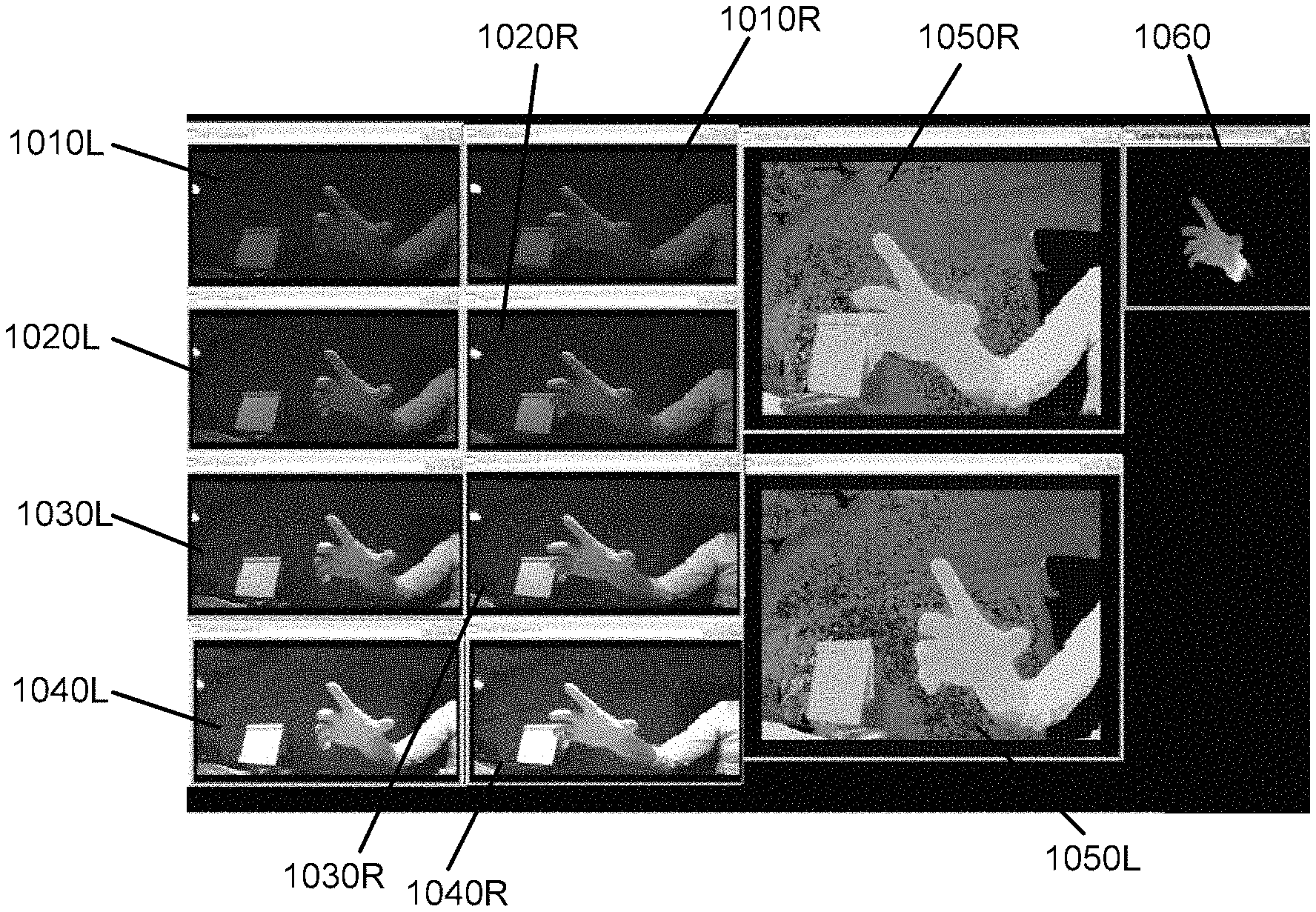
FIG. 10 shows four different source images at different exposure values; their associated reconstruction, and associated depth map;
FIG. 11 shows an example of RGB reconstruction in the presence of a light source in the image;
FIGS. 12(a) and 12(b) (collectively FIG. 12) are flowchart diagrams representing an activity diagram associated with implementation of an illuminant estimate;
FIGS. 13(a) and 13(b) depict two-dimensional cross-sections of RGB data at different light temperatures;
FIG. 14 depicts a number of three-dimensional representations of the illuminant estimation of FIG. 13 of approximately 6000K within an RGB cube;
FIGS. 15(a)-15(f) comprise a set of graphs depicting highlights of skin tone with and without white balancing under different illuminant conditions;
FIGS. 16(a) and 16(b) are graphs depicting exemplary hue and chroma profiles for metallic trim;
FIG. 17 depicts a number of exemplary histogram cases and associated irradiances and exposure settings; and
FIG. 18 is a flowchart diagram depicting a light slicing process in accordance with an embodiment of the invention.
DETAILED DESCRIPTION
One or more embodiments of the invention will now be described, making reference to the following drawings in which like reference numbers indicate like structure between the drawings.
Illuminant Estimation
Image colors may vary significantly as a function of an illuminant incident on one or more given surfaces that may be under observation. As has been recognized by the inventors of the present invention, successfully estimating this illuminant color is essential in the analysis of a given object's true color value. In accordance with one or more embodiments of the invention, it has been determined that color is inherently perceived as a function of incident illuminant light (or an ensemble of illuminant light sources) as well as the surface's relationship to that ensemble.
Chromaticity Maximization with the Camera Response Function
As noted above, the overall goal of Chromaticity maximization is to devise a means for maintaining color consistency across scenes with different lighting conditions and under different illuminants. To accomplish this goal, in accordance with one or more embodiments of the present invention, a camera response function is first computed and then used to synthetically create profiles of various pixels at different exposures. Then, the exposure that maximizes chromaticity is determined and is therefore employed in accordance with one or more embodiment of the invention.
Overview of the Camera Response Function
A camera response function relates scene radiance to image brightness. For a given camera response function the measured intensity, Z, is given by Debevec, P. E., & Malik, J. (1997). Recovering High Dynamic Range Radiance Maps from Photographs. SIGGRAPH 97: Z.sub.ij=f(E.sub.it.sub.j) Equation 1 where f encapsulates the nonlinear relationship between sensor irradiance, E, and the measured intensity of a photosensitive element (pixel) over an exposure time, t (Debevec & Malik, 1997) is given by Z.
The camera response function can be used to convert intensity to irradiance by recovering the inverse of the response, denoted as f-.sup.-1: f.sup.-1(Z.sub.ij)=E.sub.it.sub.j Equation 2 Taking the natural logarithm of both sides, g represents the inverse log function defined by: g(Z.sub.ij)=ln(f.sup.-1(Z.sub.ij))=ln(E.sub.i)+ln(t.sub.j) Equation 3
Letting Z.sub.min and Z.sub.max define the minimum and maximum pixel intensities of N pixels and P images, g can be solved by minimizing the following quadratic objective function:
.times..times..times..times..function..function..function..times..times..- times..times..lamda..times..times..times..function..times.''.function..tim- es..times. ##EQU00001##
where the first term satisfies Equation 3 and the second term imposes a smoothness constraint on the second derivative, such that: g''(z)=g(z-1)+2g(z)-g(z+1) Equation 5 The weighting function, w, is given by Granados, M., Ajdin, B., Wand, M., Christian, T., Seidel, H.-P., & Lensch, H. P. (2010), Optimal HDR reconstruction with linear digital cameras, CVPR (pp. 215-222) San Francisco: IEEE.
.function..ltoreq..times.>.times..times..times. ##EQU00002##
Once the inverse camera response function is known, a map of the scene irradiance may be obtained from P images by weighting exposures, which produce intensities closer to the middle of the response function or another targeted set of criteria in intensity, chromaticity or any combination thereof:
.times..times..times..times..function..times..function..function..times..- times..function..times..times. ##EQU00003##
For a color sensor, the camera response function may be developed separately for each channel assuming that the channels respond equally to achromatic light. This means: Z|Z.di-elect cons.{R,G,B} Equation 8 where the response is given by: R.sub.ij=f.sub.R(E.sub.t.DELTA.t.sub.j) G.sub.ij=f.sub.G(E.sub.i.DELTA.t.sub.j) B.sub.ij=f.sub.B(E.sub.i.DELTA.t.sub.j) Equation 9 and the inverse response at a common exposure is given as: g.sub.R(R.sub.ij)=ln(E.sub.Ri)+ln(.DELTA.t.sub.j) g.sub.G(G.sub.ij)=ln(E.sub.Gi)+ln(.DELTA.t.sub.j) g.sub.B(B.sub.ij)=ln(E.sub.Bi)+ln(.DELTA.t.sub.j) Equation 10 Creating Synthetic Photographs from Exposures
Once the irradiance of each of the channels is known, the log-inverse camera response function may be used to compute the response of the sensor to a user-specified exposure, .DELTA.t, creating virtual photographs from a series of observations at different exposure values. An example of this process is depicted in FIGS. 10 and 11, described below.
Hence, a set of new channels, R.sub.i, G.sub.i, B.sub.i, can be computed from an observed set of exposures, such that: R.sub.i.di-elect cons.g.sub.R(R.sub.i)=ln(E.sub.Ri)+ln(.DELTA.t) G.sub.i.di-elect cons.g.sub.G(G.sub.i)=ln(E.sub.Gi)+ln(.DELTA.t) B.sub.i.di-elect cons.g.sub.B(B.sub.i)=ln(E.sub.Bi)+ln(.DELTA.t) Equation 11 Equation 11 may be written more efficiently as: R.sub.i=g.sub.R.sup.-1(ln(E.sub.Ri.DELTA.t))=f.sub.R(E.sub.Ri.DELTA.t) G.sub.i=g.sub.B.sup.-1(ln(E.sub.Gi.DELTA.t))=f.sub.G(E.sub.Gi.DELTA.t) B.sub.i=g.sub.B.sup.-1(ln(E.sub.Bi.DELTA.t))=f.sub.B(E.sub.Bi.DELTA.t) Equation 12 Chromaticity Maximization and Color Consistency
With the ability to reconstruct images/pixels of a scene at any exposure value with an acceptable degree of accuracy, in accordance with various embodiments of the invention, a method with which one can extract the prevalent Hue value by viewing the region around the maximum Chromaticity that is associated with a given pixel is provided. Using the Camera Response Function, a method for maintaining robust color consistency throughout a scene by maximizing Chroma and plotting the values of hue that are associated with different Chroma values in the neighborhood of maximum Chroma is provided.
Maximizing Chromaticity
The exposure value(s) that maximize Chromaticity, C.sub.ij, for a given pixel, within the constraints of a camera's response function, by maximizing the Chromaticity for a pixel at location (i,j) may be provided as:
.DELTA..times..times..times..times..DELTA..times..times..times..times..ti- mes..times. ##EQU00004## where .DELTA.t.sub.ij is the exposure value that maximizes Chromaticity at location (i,j). Note that, C.sub.ij is given by (Hanbury, 2008): C.sub.ij= {square root over (.alpha..sub.ij.sup.2+.beta..sub.ij.sup.2)} Equation 14 where .alpha..sub.ij and .beta..sub.ij are given by:
.alpha..times..times..times..beta..times..times..times. ##EQU00005##
Computing the exposure that would maximize the Chromaticity in Equation 13, then calculating the hue associated therewith allows for finding a hue that is relatively constant across multiple lighting intensities of the same illuminant, since each different intensity will have a set of exposure values that is associated with it. This approach may also be extended to multiple illuminants as will be described in greater depth below, by estimating the illuminant value that is associated with a given scene.
Different Tones and their Apparent Color
Depending on an exposure value that is configured in one or more camera settings, different objects can appear to have colors that are very dissimilar from the perceived colors by observers. A problem arises in the definition of a perceived color in a field-of-view and how it relates to the colors that are associated with the object. However, observing the three channels of a pixel across a whole range of exposure values provides a better idea as to the object's true color, and not just the apparent color. Assuming that the lux that is incident at a certain scene is known, and assuming that the exposures that are associated with a given process to reconstruct lux are also known, it then becomes a significantly simpler problem to address estimation of the correct color. Hence, looking at a given set of exposure values and their associated images is a good way of identifying the different apparent colors that are associated with such images. An example Camera Response Function is presented in FIG. 1. As is shown in FIG. 1, the camera response function 110 is shown as a graph of intensity 120 versus the combined irradiance and exposure 130. The graph depicted in FIG. 3 depicts the same camera response function, broken into its component colors, red (330R), green (330G) and blue (330B) at a different exposure value. The curve of each camera response function 330R, 330G, 330B thus defines the range of irradiance 320 that can be reconstructed given the exposure value 340 and intensity 310. FIG. 4 depicts an example of irradiance sensitivity and associated histogram modes, representative of a more general example of the images shown in FIG. 3. Triangles 410, 420, 430, 440 represent ranges of good exposure recovery associated with various exposure settings, where the triangles indicate the irradiance recovered at a given pixel intensity.
Approximating the Camera Response Function with B-Splines
Another approach is to approximate the CRF with B-spline polynomials, such that a C2 continuous graph is presented. This is important to reduce the overall amount of data that is used to store the camera response function. The CRF may also be approximated with a best-fit log function.
Adding Context to Chromaticity Maximization--Dealing with Gray and Metallic Objects
Defining Relationships that are invariant to color temperature is essential to the identification of regions with high-reflectivity. Not every pixel will have high Chromaticity values; specifically pixels that are either too gray with naturally low Chromaticity, and pixels that belong to regions that are highly specular, both exhibit low Chromaticity. In photography, High Dynamic Range (HDR) imaging is used to control such cases, de-emphasizing specularities and over-exposing very dark regions. The intended consequence in both cases defines higher Chromaticity in both of these regions. We instead suggest a twist to HDR photography that not only allows it to run much faster, but makes it significantly friendlier to regions of higher Chromaticity, while de-emphasizing regions that are too bright (specular regions) or too dark. As an example, FIG. 2 highlights a case where metallic data may be perceived as highly specular. It has been determined by the inventors of the present invention that a significant amount of Chromaticity, as well as hue, can be obtained for a certain range of exposure values, albeit a small one. It is precisely for cases like these that a better understanding of hue and Chroma is needed, as well as how they are defined and what their non-zero support regions look like, specifically in the case of Chroma. As is shown in FIG. 2, hue 210, chroma 230 and intensity 220 are shown for different exposure values. It should be noted that a maximum value for each of these graphed variables is presented at particular exposure value. In FIG. 2, the maximum chroma is shown between an EV of 8 and 9 for this example.
Eliminating Reflectivity with the Camera Response Function
To identify reflectivity, it is important to address regions with such high reflectivity through the utilization of the CRF. Since colors can be returned that are associated with Exposure Values (EVs) that have been artificially enhanced. Note that the camera response function has a logarithmic nature that introduces various irradiance data reduction errors when the CRF, specifically in regions with dense irradiance information. This necessitates a non-uniform spacing of the exposures, .DELTA.t, used to reconstruct the irradiances, as illustrated in FIG. 3. When computing a maximum Chromaticity, it makes sense to try and pay special attention to regions of the CRF where irradiance information is dense, and to try and target slightly under-exposed reconstructions, especially outdoors. Irradiance sensitivity is better defined in slightly darker regions for most image sensors, allowing for a better image reconstruction. The irradiance error that is associated with the reconstruction can be calculated from the first derivative of the response function itself. Exposure settings can be chosen such that a finer quantization of the irradiance and more accuracy coincide with the most frequently repeated irradiances in the image, i.e. the statistical modes. This provides the most sensitivity at the most dominant irradiances in the field of view or region of interest, maximizing the signal to noise ratio. When the number of modes is less than the maximum number of exposures, the exposures can be placed closer together allowing the inherent averaging in the irradiance recovery to become more effective.
Irradiance Sensitivity and Exposure Settings
Looking at the CRF's first derivative, the irradiance sensitivity is maximized where the first derivative is also maximized. As an example, FIG. 5 represents a CRF 520 as well as its first derivative 525. An intensity value is shown in the vertical axis 510, while the horizontal axis of the graph in FIG. 5 shows the log-irradiance 520 that is associated with it.
The maximum sensitivity, S, in irradiance as determined by the maximum of the first derivative, occurs at approximately Z=205 or g(Z)=0.5, where g represents the inverse CRF in accordance with a particular embodiment of the invention. However, this does not mean that in all situations the value to be chosen should be 205. Rather, a constraint will preferably be put in place, as will be described below, to address image quality and bring the value down to a range that is more consistent with visually acceptable image quality. So, chroma maximization will preferably be attempted selectively, i.e. maximizing chromaticity within a given set of constraints, one of which is maximum intensity that is associated with the data. S=f'(g(z)) Equation 16
The log-exposure that produces the most sensitivity to a given irradiance can be computed as: ln(.DELTA.t)=g(arg max(f'(g(z)))-ln(E) Equation 17 Irradiance Histogram Computation
The current approach to computing the irradiance histogram via the calculation of the CRF transforms the individual red, green, and blue irradiances into a grayscale irradiance using the grayscale conversion coefficients typically applied to pixel values, Ez=0.3Er+0.59Eg+0.11Eb. If the CRF were linear, this would be equivalent to the grayscale irradiance computed by first converting the pixels to grayscale, then applying the CRF, E.sub.z=g(z)=g(0.3R+0.59G+0.11B) Equation 18 Since the CRF is non-linear, in accordance with embodiments of the invention, the grayscale irradiance should either be computed from a grayscale conversion of the demosaiced RGB values or taken directly from the Bayer pattern.
Both approaches assume that the grayscale irradiance adequately represents the per-channel irradiance. Although this assumption may be practical to simplify the process of synthetic data creation, it still discounts the fact that the differences between the irradiance channels drastically affect hue. Another option is to create an irradiance histogram over all channels simultaneously, such that the modes reflect the most dominant irradiances of all channels.
Relationship Between Modes and Exposure Settings
In an irradiance histogram, a mode may be present around one or more local maxima. As an example, FIGS. 6(a) and 6(b) (collectively FIG. 6) below represents two such cases, with one mode 610 (FIG. 6(a)) and two modes 620, 630 (FIG. 6(b)), respectively. The graphs in FIG. 6 have been constructed by calculating the irradiance histograms of the two different cases. Ideally, each mode should coincide with an exposure setting that minimizes noise at the corresponding irradiance. Exception may occur under various conditions, including: If two or more modes occur close to each other (nearly identical irradiance) while one or more smaller modes (less pixels) occur at separate, distinct irradiances. If a mode appears at zero irradiance indicating that either scene is extremely dark or the irradiance is unrecoverable.
In one exception, highlighted in FIGS. 7(a) and 7(b) (collectively FIG. 7), the exposure settings may be attached to modes occurring at independent locations. As is shown in FIG. 7, a number of local maxima 710, 720 are shown occurring in close proximity to each other. As a result, a lower number of exposure settings may be chosen, or the exposure settings may be chosen closer to each other.
Unrecoverable Irradiance
A problem with this approach occurs if the exposures that are used for computing the irradiances cannot recover certain ranges of irradiances. This can occur when the scene changes too drastically and the exposures clip or saturate one or more of the source images. One option is to set such pixels' associated irradiances to either zero or 255, representing a means with which to mitigate the associated effects. This is a reasonable assumption to make since the associated source values, i.e. from the source images at different exposure settings, are too extreme on one side of the intensity range or the other. The rationale behind this issue stems from the fact that, given proper exposures, irradiances that are deemed unrecoverable are too low, representing pixels that are near zero in intensity, and hence have very little pixel information that is associated with them. These irradiances can also be too high, i.e. representing specularities in the field of view where the pixel's intensity in one or more of the three channels is too high for the observations that are associated with an exposure range. In this case, a multilinear constraint on dichromatic planes (Toro & Funt, 2007) may be used to first estimate the illuminant and then remove illuminant effects from the scene, to prevent artificial colors from occurring. Either way, recovering the irradiance would then require more than the method that is described so far and would require an understanding of the illuminant that is associated with the scene, as well as eliminating it.
Histogram Cases
Cases of different histogram distributions, as well as the lighting conditions that are associated with them, are presented in FIG. 17. The second column depicts representative histograms of such cases, with the third column depicting four overlaid rolling exposure settings, as well as the theoretical set of exposures that can be computed via the observations and the CRF. As is shown in FIG. 17, the different histogram distributions may include any number of different possible lighting conditions. In particular, lighting conditions representing high contrast, backlit, low light, night toggle and unrecoverable are shown. As can be seen in the high contrast case, pixel responses are computed over a wide range of exposures, thus reducing the overall average response function. The exposure settings are hence set over a large range of values to cover a wider dynamic range. The second graph depicts a backlit case, with moderate contrast lighting. As can be seen, pixel responses are provided over a more limited range of exposure values, thus reducing the overall dynamic range of the scene, but increasing the average intensity over the available range. Exposure settings are similarly reduced to cover this reduced dynamic range as use of exposure settings outside of the acceptable range will fail to provide additional pixel information. This reduction in dynamic range is further shown in the third graph of FIG. 17, depicting a low lux environment in which the range of exposure values is further reduced, while still raising the overall intensity over the available dynamic range. An even further reduced dynamic range is shown in the "night toggle" state, with a corresponding higher average intensity over the dynamic range. A single exposure setting, or fewer exposure settings, may be employed to address the reduced dynamic range. Also shown are unrecoverable pixels, i.e. pixels which are too bright or too dark, over multiple exposures, to have their actual values recovered correctly. These pixels may be disregarded in the various calculations. Auto Exposure Bracketing
Auto Exposure bracketing is a means of capturing high dynamic range (HDR) images from a set of low-dynamic range images at different exposure settings. This is a prevalent technique in photography in which multiple images are taken, typically three, one with an optimal exposure setting, with a second image being taken at a lower EV value, and a third image being taken at a higher EV value. The idea is to try and get as much dynamic range of the scene as possible with a single image, and then use the other images to fill in any missing information, by over-exposing dark regions or under-exposing really bright regions.
As mentioned earlier, High Dynamic Range imaging is critical for photography. HDR is used in a number of instances. Auto-exposure bracketing techniques are very prevalent in industry (Canon U.S.A., Inc., 2012), academia (Robertson, Borman, & Stevenson, 2003), and in patents and patent applications (Yeo & Tay, 2009).
Some Common Assumptions and Weaknesses
Almost every AEB technique requires a known intensity histogram (Ohsawa, 1990). Some may also require a known irradiance histogram (Guthier, Kopf, & Effelsberg, 2012) as well. However, if the histogram is not adequately covering pertinent values in the scene, then the AEB technique will converge on the wrong settings. Also, if the histogram covers regions belonging to the background, instead of the region of interest, the AEB algorithm will converge on exposures that don't capture the dynamic range of values of the targeted ROI.
A Control Algorithm for Recovering Max Chromaticity Images
Therefore, in accordance with one or more embodiments of the present invention, a new approach that can take advantage of chromaticity maximization under resilient hue conditions, while maintaining a robust exposure bracketing algorithm is presented. This approach is depicted in FIG. 8. In step 810 the illuminant is first estimated, via an estimation of its color temperature, determined in accordance with a method presented below. Once the illuminant is estimated, the color space is preferably rectified to account for the illuminant's effects on the scene at step 820. A region-of-interest (ROI) preferably defined in the scene, and the irradiance histogram, as described above, may be computed in step 830. Exposure settings are preferably modified in step 840, per the exposure control algorithm that will be described below, and as depicted in FIG. 9. Chromaticity may then be maximized in step 850, and the various input settings (such as hue and chroma, as well as any further desired values are preferably tracked in real-time in step 860. The input settings will also be described below.
Control Algorithm for Adaptive Pixel-Based Irradiance Estimation
A control algorithm provided in accordance with one or more embodiments of the present invention can now be used to describe the scene. FIG. 9 highlights the state diagram of the control algorithm. Six states are defined in the control algorithm:
UE--Under exposed: stands for scenes that are underexposed and whose exposure values need to be increased to compensate for such a case.
OE--Over exposed: stands for scenes that are overexposed and whose exposure values need to be decreased to compensate for too much irradiance in the scene.
WE--Well-exposed: stands for scenes that are well-defined with a quality dynamic range defined by exposures that cover most of the scene.
LL--Low lux: this stands for scenes (generally under 500 Lux) with a limited dynamic range that requires fewer exposures to recover irradiance.
NM--Night mode: this is an extension of the low-lux case (under 20 Lux) where a dual mode sensor may choose to turn on infrared LEDs for operating the system. NM can be accessed from the LL or SM states.
SM--Scan mode: represents a state where the system searches through the set or subset of available exposures to optimize settings for a new scene.
In accordance with an embodiment of the invention, additionally defined transition criteria based on the presence of underexposed as well as over exposed pixels, the mean of the irradiance distribution, the support window for the hue distribution, and the overall chroma distribution are preferably employed. As is shown in FIG. 9, a more detailed overview of the different cases is provided. FIG. 9 presents a state diagram representation of the control algorithm that is used for Automatic Exposure Bracketing and exposure correction. Implementation of rolling exposures in accordance with one or more embodiments of the invention including three fundamental states Under Exposed, Well Exposed and Over Exposed, as well as Low Lux, Scan Mode, and Night Mode, is also illustrated. As is shown in FIG. 9, an image that is well exposed (WE) may transition to either under exposed (UE), over exposed (OE), low lux (LL), or stay in the its well exposed (WE) state. Any image may of course also stay in its current state. Low lux (LL) images may be transitioned to night mode (NM) which will persist until the image is transitioned to well exposed (WE). All states may transition to a scan mode (SM) (except from night mode (NM). Once the scan is completed, the image will transition to either well exposed (WE) or night mode (NM). Thus, depending on various threshold conditions, the AEB state machine will transition between the various states. The AEB state machine will also vary the exposure value spacing, number of exposures, as well as the thresholds themselves, depending on the state. Note that in FIG. 9, very low irradiances are truncated to zero, and very high irradiances are truncated to 255, denoted as b0 and b255 respectively.
Example Source and Output Images
As an example, FIG. 10 depicts an embodiment in which four images are captured at different exposure values. As is shown, a first pair of images 1010L, 1010R is taken by a pair of stereo cameras at a first exposure value. Next, a second pair of images 1020L, 1020R are taken, preferably by the same pair of stereo cameras, As is further shown in this particular embodiment, third and fourth pairs of images 1030L, 1030R and 1040L, 1040R are also taken. Of course, any particular desired number of images may be employed. Furthermore, a single or multiple cameras may be employed for each set of images at each exposure level. The four left images (or any desired subset thereof) may then be employed to reconstruct image 1050L, while the four right images (or any subset thereof) may then be employed to reconstruct image 1050R. Finally, these reconstructed images are then presented using the camera response function and observations from all of the capture images in accordance with the method noted above, and a depth map 1060 is preferably generated.
A second example is shown in FIG. 11. In FIG. 11, depth is possible to be reconstructed despite the presence of a direct light source in the field-of-view. The light source's is minimized and the rolling exposures help compute the most suitable chromaticity-maximized value. Similar to FIG. 11, a first pair of images 1110L, 1110R are taken by a pair of stereo cameras at a first exposure value. Next, a second pair of images 1120L, 1120R are taken, preferably by the same pair of stereo cameras, As is further shown in this particular embodiment, third and fourth pairs of images 1130L, 1130R and 1140L, 1140R are also taken. Of course, any particular desired number of images may be employed. Furthermore, a single or multiple cameras may be employed for each set of images at each exposure level. The four left images (or any desired subset thereof) may then be employed to reconstruct image 1150L, while the four right images (or any subset thereof) may then be employed to reconstruct image 1150R. Finally, these reconstructed images are then presented using the camera response function and observations from all of the capture images in accordance with the method noted above, and a depth map 1160 is preferably generated.
Ensembles of Illuminants for a Given Scene and their Temperature Estimation
Estimating the illuminant is critical to accounting for it in a given scene and correcting the RGB color space, per the effects of the illuminant (Gijsenij, Gevers, & Weijer, 2011). Black body radiators are ones that emit light when excited at different temperatures. One can look at regular light sources as black body radiators. These vary from red to white, according to the temperature that is associated with their light color, in Kelvins. Typical temperature ranges vary from 2000K (red) to 9000K (blue/white or white with blue tint).
A set of illuminants may be defined based on values that are associated with their respective color temperatures (usually defined in Kelvins). In a manner similar to what has been defined in (Barnard, Cardei, & Funt, 2002), each illuminant may be defined according to its Chromaticity map, and may be expanded to include a more substantive set of illuminants. As a result, to find an approximate illuminant, the Veronese map of degree n may be computed, such that c(x).sup.Tv=0 Equation 19 where c(x) is an observed color belonging to a single material and v is a normal vector associated with the dichromatic plane of the material. The projection of the observed color is projected as: d(x;w).sup.T=M(w).sup.Tc(x) d(x;w)=M(w).sup.Tc(x) Equation 20 where w is a vector representing the color of the illuminant and d(x;w) represents the projection of the observed color c(x) onto a 2-D subspace using the 3.times.2 projection matrix M(w). The 2-D subspace is orthogonal to the light vector. d(x;w).sup.Tu=0 Equation 21 where u is a vector in the 2-D subspace that consists of the coefficients of a linear combination.
.times..times..function..times..times..times..times..times..function..tim- es..times..times..times. ##EQU00006## where v.sub.n(d)=[d.sub.1.sup.nd.sub.1.sup.n-1d.sub.2.sup.1d.sub.1.sup.n-2d.sub- .2.sup.2 . . . d.sub.2.sup.n].sup.T u.sub.i is one vector in a collection of n vectors that represent all of the materials in the scene. v.sub.n(d)=[d.sub.1.sup.nd.sub.1.sup.n-1d.sub.2.sup.1d.sub.1.sup.n-2d.sub- .2.sup.2 . . . d.sub.2.sup.n].sup.T Equation 23 where d.sub.1 and d.sub.2 are the 2-D coordinates of the projected color onto the subspace that is orthogonal to the light vector and v.sub.n(d) is the Veronese map of degree n and n is the number of materials in the scene.
.LAMBDA..function..function..function..function..function..function..time- s..times. ##EQU00007## where .LAMBDA..sub.n consists of the Veronese maps for all of the colors under consideration.
.times..times..times..times..times..times..times..times..times..times..fu- nction..times..times..times. ##EQU00008##
Equation 25 can now be rewritten as:
.times..times..times..LAMBDA..times..LAMBDA..times..times..times. ##EQU00009## where a.sub.n is the set of coefficients associated with each Veronese map in .LAMBDA..sub.n. As mentioned in, Toro, J., & Funt, B. B. (2007). A multilinear constraint on dichromatic planes for illumination estimation. IEEE Trans. Image Processing, 16 (1), 92-97, a candidate color, w, is the actual color of the light if the smallest eigenvalue of matrix, .LAMBDA..sub.n.sup.T.LAMBDA..sub.n, is equal to zero. Hence, the approximate illuminant is identified as the one corresponding to the smallest eigenvalue. To choose from the different materials, one approach can be applied where scenes are subdivided into various regions, based on both color as well as texture. A system for performing this approach may comprise any number of region classification schemes, and in a preferred embodiment, a system such as that described in U.S. patent application Ser. No. 12/784,123, currently pending, the contents thereof being incorporated herein by reference. Hence, an image is preferably broken up into regions of dominant texture or color, with multiple segments representing different blocks of data being present in any given image. For each block, the illuminant estimation process is conducted, such that the temperature of the illuminant is computed, as well as the associated RGB values. The color space of the image is then rectified to mitigate the illuminant's effects. The rest of the software stack follows from this step, to reconstruct segments followed by depth reconstruction, as described in U.S. patent application Ser. Nos. 12/784,123; 12/784,022; 13/025,038; 13/025,055; 13/025,070; 13/297,029; 13/297,144; 13/294,481; and 13/316,606, the entire contents of each of these application being incorporated herein by reference. Example Approach to Illuminant Estimate
Referring next to FIGS. 12(a) and 12(b) (in combination referred to as FIG. 12), an approach to illuminant estimation is described, as presented in (Toro & Funt, 2007) and adapted here in accordance with the various embodiments of the invention. As is shown in FIG. 12, at step 1210, a desired number of candidate illuminant estimates as well as their desired color temperatures may first be configured. The blackbody radiator color may then be obtained at step 1215. The color is then preferably converted from CIE XYZ to RGB at step 1220. On an image level, the total number of materials as well as the block size that is associated with each material may also be configured, and therefore, at step 1225 it is questioned whether the process has been performed for all (or substantially all) desired candidate illuminants. If this inquiry is answered in the negative, and it has therefore been determined that not all of the desired candidate illuminants have been considered, processing preferably returns to step 1215, and processing for a next desired illuminate candidate begins.
If the inquiry at step 1225 is instead answered in the positive, and it is therefore determined that all desired candidate illuminants have been considered, processing then passes to step 1230 where the number of materials and block size are configured. Next, at step 1235, a projection matrix for the two-dimensional subspace orthogonal to a light vector may be computed, preferably employing the relevant equations described above. Then for each pixel defined in the two dimensional subspace, at step 1240, the pixel color is then preferably projected onto the subspaces of illuminants preferably according to Equation 5 described above, and at step 1245 a Veronese map from the result of the projections may then be computed, preferably employing Equation 8 noted above. Processing then continues to step 1250 where it is questioned whether the processing associated with steps 1240 and 1245 has been performed for each pixel (or substantially each pixel) in a defined block, or section of the image under observation. If this inquiry is answered in the negative, and it is determined that processing has not been completed for all desired pixels, processing returns to step 1240 for addressing a next pixel.
If on the other hand, if the inquiry at step 1250 is answered in the affirmative, and it is therefore determined that processing has been completed for all desired pixels, processing then passes to step 1255, where a matrix is preferably then built from the Veronese projections of all the pixels in a given block of the image, preferably employing Equation 10 described above. At a next step 1260, the resultant matrix is then multiplied by its transpose, the eigen values of the results being computed, and the smallest eigenvalue is obtained, preferably in accordance with Equation 11 described above. Processing then passes to step 1265 where it is questioned whether processing for all desired candidate illuminants (or substantially all desired candidate illuminants) for the current block has been completed. If the inquiry at step 1265 is answered in the negative, and therefore it is determined that processing has not been completed for all desired candidate illuminants for the current block, processing returns to step 1235 for a next of the desired candidate illuminant values for the current block.
If on the other hand, the inquiry at step 1265 is answered in the affirmative, thus confirming that processing has been completed for all of the desired candidate illuminants for the current block, processing then passes to step 1270 where the relative error is preferably computed for each illuminant by dividing the smallest eigenvalue of each illuminant by the eigenvalue of the set. Processing then passes to step 1275, where it is questioned whether processing for all blocks (or substantially all blocks) in the image has been completed. If this inquiry is answered in the negative, and it is therefore determined that processing for all blocks in the image has not been completed, processing once again returns to step 1235 for a next block in the image.
If on the other hand the inquiry at step 1275 is answered in the affirmative, and it is therefore determined that processing for all blocks in the image has been completed, processing then passes to step 1280 where an illuminant that minimizes relative error across all of the blocks is chosen.
Many other variants to this approach are contemplated in accordance with the various embodiments of the invention. For the sake of consistency and to enable visualization, the next following description should be considered applicable to two-dimensional as well as three-dimensional visualizations of the resultant light vectors in RGB space, while the three-dimensional implementation will be described.
Three-Dimensional Visualization of the Light Vector Relative to the RGB Space
Referring next to FIGS. 13(a) and 13(b) (collectively FIG. 13), image RGB data is shown as plotted on an RGB cube. In each plot in FIG. 13, a light vector is also plotted as a two-dimensional projection of the RGB cube onto a surface upon which all the data would lie. Different projections of the RGB data onto the light vector are highlighted here at different temperature settings representative of 18 different illuminant surfaces having illuminant color temperatures varying from 2000K to 10500K. Also, a single RGB cube at 6000K, shown in FIG. 14 from different perspectives, highlights the spread of the illuminant estimates for the individual pixels as well as the dominant direction of the illuminant that is associated with them, under an illuminant, defined by its color temperature, in Kelvins. Per the discussion that has been presented earlier, the smallest spread is presented as the most accurate approximation of the correct illuminant.
Integration of Exposure Bracketing Features into Segmentation
As noted above, one potential problem that is associated with segmentation under challenging lighting conditions is that of maintaining color consistency as pixels are being tracked in a field-of-view. In accordance with one or more embodiments of the present invention, through the user of Chroma maximization, color consistency can be achieved and maintained even as color constancy is no longer plausible throughout a scene. A clear distinction should be drawn between color constancy, i.e. maintaining a constant color across the entire span of frames, and color consistency, where a given color is allowed to change, but not across adjacent frames. By computing max Chroma through simulating row lines or exposure values, one can now move on to the problem of segmentation. Specifically, given that different objects may appear with a similar hue or even Chroma under similar lighting conditions, it is left to the use and manipulation of exposure settings to identify differences in different materials and the way that such differences may be exploited in segmentation. In accordance with one or more embodiments of the invention, quality of color-based segmentation accuracy can be accomplished by computing which exposure value(s) would provide for Chroma maximization, per the description of the Camera Response Function at different irradiances. Not only can segmentation now be accomplished based on texture and color as described in U.S. patent application Ser. Nos. 12/784,123; 12/784,022; 13/025,038; 13/025,055; 13/025,070; 13/297,029; 13/297,144; 13/294,481; and 13/316,606, the entire contents of each of these application being incorporated herein by reference, wherein both texture and color are used to segment in stereo images, but one can also define or profile the evolution of such a color across multiple exposure settings, given only a few observations. Such information is then preferably integrated into segmentation and used to further enhance pixel and segment-level discriminability. Thus, a pixel may be classified and clustered by its response at different exposures.
Light Slicing
Referring next to FIG. 18, One relevant observation about different scenes is that objects have redundant information across multiple light frequencies, and hence multiple exposures. Exploiting this property allows one to methodically decompose the scene based on the luminance that is associated with the different exposure settings. Therefore, in accordance with one or more embodiments of the present invention, in order to simplify the depth computation problem, as described in one or more of as described in U.S. patent application Ser. Nos. 12/784,123; 12/784,022; 13/025,038; 13/025,055; 13/025,070; 13/297,029; 13/297,144; 13/294,481; and 13/316,606, the entire contents of each of these application being incorporated herein by reference, one may approach depth computation by "light slicing" the scene, i.e. exposing the scene at different time intervals, rendering the scene, and then computing depth on the regions that have been rendered. Once depth is computed on the rendered regions, then the exposures are preferably set again to brighten the image. After once again exposing the scene, once again this depth computation process is undertaken, but only new pixels that have appeared in the now brighter image preferably will have their depth computed. The process is terminated once all of the pixels have been marked, or after a desired number exposure jumps have been employed. Thus, as is shown in FIG. 18, an EV value is first incremented at step 1810 and at step 1820 the scene is rendered. At step 1830, any new components or pixels are rendered, and at step these new pixels are integrated with an existing depth map. At step 1850 it is inquired whether there are additional EV values to be employed. If so, processing returns to step 1810. If all desired EV values have been employed, processing passes to step 1860 where a final depth map is rendered.
Color Consistency Towards Feature Constancy
One can now start to look at what features to extract from better discriminability and color quality. These features are presented below, as determined by the inventors of the present invention:
1. Prevalent or Persistent Hue Value:
A prevalent or persistent hue can be extracted from the Chroma maximization graphs that are associated with the camera response functions of the R, G, and B channels, (see FIG. 15 and FIG. 16 for examples). FIGS. 15(a)-15(f) (collectively FIG. 15) depict highlights of skin tone without white balancing (first row) and with white balancing (second row) under different illuminant and environmental conditions, described and depicted earlier, and including different illuminants, associated with different light temperatures and the like. As can be seen in FIG. 15, there is present a number of very clear distinguishable features, such as a prevalent hue value, and the presence of a Chromaticity peak value within the support window of the hue value. In fact, hue is resilient and consistent across multiple exposures. FIG. 16 depicts an example of hue/Chroma profiles for metallic trim. Note the difference in the profiles, especially relative to skin tone for metallic surfaces and matte surfaces. This is because different materials will respond differently when exposed at different levels of exposures, and hence the images that are subtended at the different exposures will inherently be different as well, when they are evaluated as a whole. This concept refers to the creation of a profile of hue values at different exposure levels. This notion lends itself to the prior described notion of color consistency or prevalent/consistent hue value, with one major difference between this concept and that of color constancy: color constancy algorithms don't take into account the fact that different regions/materials/black body radiators that are illuminated in the field-of-view by the same illuminant (or different illuminants) may exhibit similar color characteristics. This is especially exacerbated through exposure bracketing (Yeo & Tay, 2009) (Ohsawa, 1990), where a system adaptively changes the set of rolling exposures, based on a set of pre-existing illumination criteria. Exposure bracketing can then lead to hue/Chroma values being reconstructed that may be extremely different from perceptually acceptable ones, or at least those that are perceptually perceived by people in a subjective test. This is quite acceptable since the notion of color constancy in human beings is deeply rooted in hierarchical scene organization, and can't be simply ported over to machines, even ones that do respect Gestalt principles of scene organization. Instead, a different hue metric--the prevalent hue value that is associated with the Chroma maximization graph at different exposures, is proposed. Using such a metric, one can define a hue that is consistently prevalent and robust across a range of exposures. This approach makes the hue estimation significantly more robust to outliers. Typical color hues will exhibit a relatively wide support function/region, (see FIG. 16) in the area of prevalent color, for various EV values, denoting what humans may perceive as color constancy. The width, or the support, of that function may differ, depending on lighting/irradiance conditions. Any method to extract the prevalent hue by treating the graph as a simple one-dimensional graph, and extracting such a prevalent hue is acceptable in this case. Without limitation, we can mention first and second-order moments, support vector machines, and a principle component analysis as among such methods. A simple best-fit curve may also work.
2. Chroma Profile/Max Chromaticity Identification and The Notion of False Colors:
Typical surfaces with good color quality exhibit good Chroma responses at a range of exposure settings, and may possibly be approximated with a Gaussian curve centered around an optimal exposure. This is especially true for skin tone, where skin tone modeling in the past has focused on Gaussian Mixture Models. For good colors well within a camera's dynamic range, and with adequate lighting, a large support window of high Chromaticity is typically the case (see FIG. 16, for example). On the other hand, over-exposing and under-exposing highly reflective surfaces as well as dark surfaces will typically generate very different responses, and produce what we are referring to in this work as false colors. Such colors' Chromaticity will typically increase with pixel intensity, i.e. exposure values that over-expose the image. Exceptions occur with illuminants whose temperature ranges are warmer (yellow or red). In such cases, black objects may exhibit high chroma settings, consistent with the scene illuminant or light source, or even consistent with the sensor's spectral response for different frequencies of light. As a result, values of Chroma for false colors, i.e. colors that are either generated by the illuminant portion of the field-of-view or by the sensor's spectral response, continually keep increasing. To counter such effects, one can also look at the Chromaticity curve under different exposure conditions. Of particular importance is the range of Chromaticity that produces reliable hue. Hence, a range of exposure values that represent a range of admissible Chroma can be used, as well as the maximum Chroma value, and its location relative to the non-zero support of the Chromaticity range. Hence, profiling Chroma vs. exposure values presents yet another critical piece to the puzzle.
3. Illuminant Estimate:
It now becomes critical to divide up the scene into regions of relatively constant illuminant estimates. Breaking up the scene into ensembles of illuminants has been presented above. However, here, the contribution of an illuminant ensemble map to the computation of depth in a field-of-view is also presented and integrated into the process that has been defined to compute overall depth. One can also mitigate the effects of a given illuminant in the scene. Illuminant estimation for an example illuminant estimation approach has been described above.
4. Irradiance:
As disclosed above, irradiance is a measure of reconstructed brightness incident on a particular pixel in an image. It can be used to detect the amount of light in a scene. Irradiance is also used to compute the maximum Chroma as well as the hue values that are associated with a given pixel. Irradiance is also used for detecting a given feature's constancy in the scene.
Putting it all Together
A novel technique for pixel superresolution is therefore provided in which multiple pixels can be extracted from a smaller number of observations. A multi-dimensional feature vector, v, is given by: v={h,c,i,t} Equation 27 Where h represents the hue feature vector, c represents the Chromaticity feature vector, i represents the irradiance feature vector, and t represents texture as a feature vector. All of these vectors have been described earlier with the exception of t, the texture feature vector. However, using texture has been defined extensively in earlier works by the assignee of the present application, as noted above. Extraction of Feature Vectors
One of the challenges that is facing all of segmentation is the capability to accurately organize the scene by means of color quality, and texture features, such that different regions in the scene can be organized via color/texture characteristics either in the spatial or frequency domain. Motion features can also be extracted to increase scene segmentation. In accordance with the various embodiments of the invention, the inventors therefore propose an entirely novel approach to scene segmentation through pixel superresolution via features that are extracted from the camera response function.
The above-described process may also be generally applicable to photography, allowing for a high accuracy HDR type process producing images as well as videos with more vivid colors, and less sensitive to difficult lighting conditions.
Application--High Dynamic Range Video and Photography
Given all of the features and the segmentation components presented above, users have the ability to interactively enable HDR features with this approach. Alternatively, an HDR video scheme can be developed that utilizes the various features that have been described above. Specifically, regions of common synthetic exposures may be exposed more uniformly, and various stable segments may be under of over-exposed based on selection criteria defined by the user. Users can also autofocus on different parts of the video in real-time, given that every component of the video is being tracked in real-time.
5. Conclusions
A novel approach to AEB as well as segmentation and disparity computation has been presented that takes into account the utilization of the Camera Response Function to synthetically create different images, maximize chromaticity, and create a notion of color consistency. This is used to produce a robust segmentation/disparity estimation algorithm. Illuminant estimation may also be used for compensating color differences that are impacted by the effect of incident illuminants. The approach has multiple other applications include HDR photography and real-time HDR video.
Furthermore, while the invention has been primarily described related to a general imaging system, the various embodiments of the invention may also be applicable to any other platform that may be used for imaging, including but not limited to mobile devices, devices employing a Graphical Processing Unit (GPU), display on 3D screens, display on 2D screens, various types of photography employing one or multiple single frame or video cameras, and the like.
It will thus be seen that the objects set forth above, among those made apparent from the preceding description, are efficiently attained and, because certain changes may be made in carrying out the above method and in the construction(s) set forth without departing from the spirit and scope of the invention, it is intended that all matter contained in the above description and shown in the accompanying drawings shall be interpreted as illustrative and not in a limiting sense.
It is also to be understood that this description is intended to cover all of the generic and specific features of the invention herein described and all statements of the scope of the invention which, as a matter of language, might be said to fall there between.
* * * * *
References
D00000
D00001
D00002
D00003
D00004
D00005
D00006
D00007
D00008
D00009
D00010
D00011
D00012

D00013

D00014

D00015

D00016

D00017

D00018

D00019

D00020

D00021

D00022

D00023

D00024

D00025

M00001

M00002
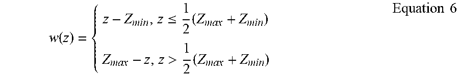
M00003
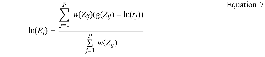
M00004

M00005
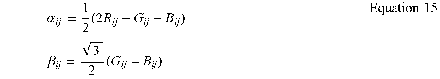
M00006

M00007

M00008

M00009

XML
uspto.report is an independent third-party trademark research tool that is not affiliated, endorsed, or sponsored by the United States Patent and Trademark Office (USPTO) or any other governmental organization. The information provided by uspto.report is based on publicly available data at the time of writing and is intended for informational purposes only.
While we strive to provide accurate and up-to-date information, we do not guarantee the accuracy, completeness, reliability, or suitability of the information displayed on this site. The use of this site is at your own risk. Any reliance you place on such information is therefore strictly at your own risk.
All official trademark data, including owner information, should be verified by visiting the official USPTO website at www.uspto.gov. This site is not intended to replace professional legal advice and should not be used as a substitute for consulting with a legal professional who is knowledgeable about trademark law.