Completions index analysis
James , et al. A
U.S. patent number 10,385,670 [Application Number 15/222,426] was granted by the patent office on 2019-08-20 for completions index analysis. This patent grant is currently assigned to EOG RESOURCES, INC.. The grantee listed for this patent is EOG RESOURCES, INC.. Invention is credited to Oscar A. Bustos, Evan Daniel Gilmore, Christopher Michael James, Eric Robert Matus.

View All Diagrams
| United States Patent | 10,385,670 |
| James , et al. | August 20, 2019 |
Completions index analysis
Abstract
A method for determining a hydrocarbon-bearing reservoir quality prior to a hydraulic fracture treatment based on completions index is disclosed. The method comprises a step performing a test determining a hydraulic pressure at which a hydrocarbon-bearing reservoir will begin to fracture by pumping a fluid in a wellbore, wherein the wellbore extends from a surface to the reservoir and the wellbore has one or more perforations in communication with reservoir; a step generating a pressure transient in the wellbore, the pressure transient travels from the surface to the reservoir through the perforations and reflects back the surface after contacting the reservoir; a step measuring response of the pressure transient at sufficiently high sampling frequency; a step determining fracture hydraulic parameters of the perforations and the reservoir using the measured response; and optimizing a stimulation treatment to the reservoir based on the determined fracture hydraulic parameters.
| Inventors: | James; Christopher Michael (San Antonio, TX), Bustos; Oscar A. (San Antonio, TX), Gilmore; Evan Daniel (Forth Worth, TX), Matus; Eric Robert (Midland, TX) | ||||||||||
|---|---|---|---|---|---|---|---|---|---|---|---|
| Applicant: |
|
||||||||||
| Assignee: | EOG RESOURCES, INC. (Houston,
TX) |
||||||||||
| Family ID: | 57276682 | ||||||||||
| Appl. No.: | 15/222,426 | ||||||||||
| Filed: | July 28, 2016 |
Prior Publication Data
| Document Identifier | Publication Date | |
|---|---|---|
| US 20160333684 A1 | Nov 17, 2016 | |
Related U.S. Patent Documents
| Application Number | Filing Date | Patent Number | Issue Date | ||
|---|---|---|---|---|---|
| 14526288 | Oct 28, 2014 | ||||
| Current U.S. Class: | 1/1 |
| Current CPC Class: | E21B 43/26 (20130101); E21B 49/008 (20130101) |
| Current International Class: | E21B 43/26 (20060101); E21B 49/00 (20060101) |
References Cited [Referenced By]
U.S. Patent Documents
| 4783769 | November 1988 | Holzhausen |
| 4802144 | January 1989 | Holzhausen et al. |
| 5031163 | July 1991 | Holzhausen et al. |
| 5081613 | January 1992 | Holzhausen |
| 5170378 | December 1992 | Mellor et al. |
| 5278758 | January 1994 | Perry |
| 5345077 | September 1994 | Allen et al. |
| 5679323 | October 1997 | Menz |
| 7100688 | September 2006 | Stephenson et al. |
| 7313481 | December 2007 | Moos et al. |
| 2005/0216198 | September 2005 | Craig |
| 2009/0255731 | October 2009 | Backhaus et al. |
| 2010/0218941 | September 2010 | Ramurthy et al. |
| 2010/0314104 | December 2010 | Shokanov et al. |
| 2011/0011595 | January 2011 | Huang et al. |
| 2011/0209871 | September 2011 | Le |
| 2011/0259581 | October 2011 | Bedouet et al. |
| 2012/0179444 | July 2012 | Ganguly et al. |
| 2012/0228027 | September 2012 | Sehsah |
| 2012/0253770 | October 2012 | Stern |
| 2012/0285744 | November 2012 | Bernard |
| 2013/0186688 | June 2013 | Rasmus et al. |
| 2013/0176139 | July 2013 | Chau |
| 2014/0060819 | March 2014 | Pindiprolu |
| 2014/0145716 | May 2014 | Dirksen et al. |
| 2015/0159477 | June 2015 | Lecerf et al. |
| 2015/0176403 | June 2015 | Chen et al. |
| 2016/0115780 | April 2016 | James et al. |
| 2016/0245073 | August 2016 | Hansen |
Other References
|
Terry O. Anderson et al., A Study of Induced Fracturing Using an Instrumental Approach, Journal of Petroleum Tecnology, pp. 261-267 (1967). cited by applicant . Mohamed S. Ghidaoui et al., A Review of Water Hammer Theory and Practice, Applied Mechanics. vol. 58, pp. 49-76 (2005). cited by applicant . Tadeusz W. Patzek et al., Lossy Transmission Line Model of Hydrofractured Well Dynamics, Journal of Petroleum Science and Engineering, vol. 25, pp. 59-77 (2000). cited by applicant . International Search Report & Written Opinion, PCT/US2015/048714, dated Jan. 19, 2016. cited by applicant . International Preliminary Search Report (IPRP) PCT/US2015/48714 dated Nov. 23, 2016. cited by applicant. |
Primary Examiner: Seo; Justin
Assistant Examiner: Royston; John M
Attorney, Agent or Firm: Winston & Strawn LLP
Parent Case Text
CROSS-REFERENCE TO RELATED APPLICATION
This application is a continuation-in-part of U.S. Nonprovisional application Ser. No. 14/526,288, filed Oct. 28, 2014, the entirety of which is herein incorporated by reference.
Claims
What is claimed is:
1. A method for determining a hydrocarbon-bearing reservoir quality comprising: performing a test determining a hydraulic pressure at which a hydrocarbon-bearing reservoir will begin to fracture by pumping a fluid in a wellbore, wherein the wellbore extends from a surface to the reservoir and the wellbore has one or more perforations in communication with the reservoir; generating a pressure transient in the wellbore, the pressure transient traveling from the surface to the reservoir through the perforations and reflecting back to the surface after contacting the reservoir; measuring the response of the pressure transient at a sampling frequency, wherein the measured response includes pressure measurement over a period of time; and determining a hydraulic parameter of the perforations, wherein the step of determining a hydraulic parameter of the perforations includes transforming the measured response to produce a transformed response, wherein the step of transforming includes providing a window having a time duration that is shorter than the period of time in the measured response, applying the window to the measured response to encompass a portion of the measured response, and determining maximum and minimum pressure in the measured response encompassed by the window, and; calculating rate of decay of the transformed response.
2. The method of claim 1, wherein the step of transforming the measured response further comprises calculating the difference between the maximum pressure and the minimum pressure.
3. The method of claim 2, wherein the difference is produced as part of the transformed response.
4. The method of claim 1, wherein the time duration of the window is 1 second.
5. The method of claim 1, the step of transforming the measured response further comprises sliding the window over the measured response at an increment of time to transform the entire measured response.
6. The method of claim 5, wherein the step of transforming the measured response further comprises determining maximum and minimum pressure in the portion encompassed by the window for each increment of time.
7. The method of claim 6, wherein the step of transforming the measured response further comprises calculating the difference between the maximum pressure and the minimum pressure in the portion encompassed by the window for each increment of time.
8. The method of claim 7, wherein the differences are produced as part of the transformed response.
9. The method of claim 5, wherein the increment of time is 0.01 second.
10. The method of claim 1, wherein the step of calculating rate of decay of the transformed response comprises finding peaks of the transformed response and fitting an exponential decay to the peaks.
11. The method of claim 1, wherein the method further comprises calculating a reflection half-life from the rate of decay.
12. The method of claim 11, wherein the method further comprises correlating the reflection half-life to a modeled hydraulic resistance.
13. The method of claim 12, wherein the modeled hydraulic resistance is obtained from adjusting an element of an electrical model representing the wellbore over a range of values.
14. The method of claim 13, wherein the element is a resistor.
15. The method of claim 1, wherein the measured response provides pressure information over a period of time and the transformed response provides pressure information different from the pressure information provided by the measured response over the same period of time.
16. The method of claim 15, wherein the pressure information provided by the transformed response includes a plurality of peaks and the rate of decay is calculated based on the peaks.
17. The method of claim 1, wherein the hydraulic parameter is flow resistance.
18. The method of claim 1, wherein the sampling frequency is more than 2 Hz.
19. The method of claim 1, the step of transforming the measured response further comprises applying the window to the measured response at an increment of time to encompass a next portion of the measured response.
20. The method of claim 19, wherein the step of transforming the measured response further comprises determining maximum and minimum pressure in the next portion of the measured response encompassed by the window.
Description
FIELD OF THE INVENTION
The present invention relates to a method for determining a hydrocarbon-bearing reservoir quality, and in particular, to a method for determining a hydrocarbon-bearing reservoir quality prior to a hydraulic fracture treatment based on a completions index.
BACKGROUND OF THE INVENTION
Hydraulic fracturing is a technique of fracturing rock formations by a pressurized fluid in order to extract oil and natural gas contained in the formations. A fluid, which usually is water mixed with sand and chemicals, is injected into a wellbore under considerable pressure to create fractures in the formations. When the pressure is removed from the wellbore, the sand props the fractures open allowing the oil and gas contained in the formations to more readily flow into the well for extraction. This technique has revolutionized oil and gas development, especially is shale formations, because it permits extraction of formerly inaccessible hydrocarbons. As a result, it has helped push U.S. oil production to a new high and generate billions of revenues to mineral rights owners, oil companies, as well federal, state, and local governments.
Hydraulic fracturing, however, can be a very expensive process, especially if the quality of the formations is unknown, in a horizontally drilled oil well, hydraulic fracturing generally is performed in several stages along the horizontal portion of the well. Typically, the horizontal portion of the well is stimulated in stages about every 200 to 250 feet. Although the horizontal portion of the well generally extends through a given hydrocarbon hearing formation, the lithology or rock quality may vary along the length of the wellbore. When oil companies conduct a frac treatment at a section of the formations that is sub-optimal, the stimulation may be ineffective or produce marginal gains in productivity for that particular stage. Assuming that the average cost for each hydraulic fracture treatment is approximately $100,000 and that some formations may have up to 80% of its sections be sub-optimal, the cost and time spent in fracturing sub-optimal sections or in determining whether to move onto another section can be substantial. In one year, an energy consulting company estimated that about $31 billion was spent in sub-optimal fracturing across 26,100 U.S. oil wells.
Moreover, even if the oil drilling companies treat a section of the formation that happens to be optimal, the treatments may not have been the optimal size. In other words, the treatment may have been too small given the favorable rock qualities that existed for that particular stage and that the well could have been even more productive and the return on the investment of the stimulation could have been even higher had a larger stimulation been pumped, or had a different stimulation fluid or amount of proppant been pumped. As such, knowing the quality of the formations prior to a hydraulic fracture treatment is beneficial to stimulation treatments.
A method called Distributed Fiber Optic Sensing has been developed to provide this information. This method is based on either temperature or acoustic sensing. In the method based on temperature sensing, a unit including a laser source and a photodetector is placed on the surface and a glass fiber is permanently installed in the well. The laser source sends laser pulses down the glass fiber and the temperature of the formations can affect the glass fiber and locally change the characteristics of light transmission in the glass fiber. The photodetector measures the laser light reflections from different spots in the glass fiber due to the temperature and the spectrum of the laser light reflections can used to determine the properties of the formations. The method based on acoustic sensing is similar to the temperature sensing one except that this method employs a unit that includes an acoustic signal generator and an acoustic signal receiver and that this method measures the reflected acoustic signals based on the strain or pressure of the formations exerted on and along various points of the glass fiber. The measured acoustic signals may have various amplitude, frequency, and phase attributes that can also be used to determine the properties of the formations.
The Distributed Fiber Optic Sensing method, however, has several drawbacks. First, this method requires running a glass fiber into the well that complicates the installation process. Second, this method usually costs around $600,000 to implement and the investment is only for one single well and is permanent. Third, this method is not economically practical on smaller reservoir wells. Fourth, to protect the fragile glass fiber, the glass fiber is typically placed within a stainless steel sheath that can attenuate the temperature or strain response, reducing accuracy of the measurement.
Accordingly, there is a need for an improved method for determining the quality of the rock formations prior to a hydraulic fracture treatment.
SUMMARY
In accordance with one embodiment of the present invention, a method for determining a hydrocarbon-bearing reservoir quality is described. The method may comprise performing a test determining a hydraulic pressure at which a hydrocarbon-bearing reservoir will begin to fracture by pumping a fluid in a wellbore, wherein the wellbore extends from a surface to the reservoir and the wellbore has one or more perforations in communication with the reservoir; generating a pressure transient in the wellbore, the pressure transient traveling from the surface to the reservoir through the perforations and reflecting back to the surface after contacting the reservoir; measuring the response of the pressure transient at a sufficiently high sampling frequency; and determining a hydraulic parameter of the perforations by transforming the measured response to produce a transformed response and calculating rate of decay of the transformed response.
In a preferred embodiment, the step of transforming the measured response may comprise generating a window defining a period of time over the measured response. This step may also comprise determining maximum and minimum pressure in the period of time defined by the window. This step may further comprise calculating the difference between the maximum pressure and the minimum pressure. The difference may be produced as part of the transformed response. The window may define a period of 1 second. Moreover, this step may comprise sliding the window over the measured response at an increment of time to transform the entire measured response.
In a preferred embodiment, the step of transforming the measured response may comprise determining maximum and minimum pressure in the period of time defined by the window for each increment of time. This step may also comprise calculating the difference between the maximum pressure and the minimum pressure for each increment of time. The differences may be produced as part of the transformed response. The increment of time may be 0.01 second.
In a preferred embodiment, the step of calculating rate of decay of the transformed response may comprise finding peaks of the transformed response and fitting an exponential decay to the peaks.
In a preferred embodiment, the method may further comprise calculating a reflection half-life from the rate of decay. The reflection half-life may be correlated to a modeled hydraulic resistance. The modeled hydraulic resistance may be obtained from adjusting an element of an electrical model representing the wellbore over a range of values. The element may be a resistor.
In a preferred embodiment, the measured response may provide pressure information over a period of time and the transformed response may provide pressure information different from the pressure information provided by the measured response over the same period of time. The pressure information provided by the transformed response may include a plurality of peaks and the rate of decay is calculated based on the peaks.
In a preferred embodiment, the hydraulic parameter may be flow resistance.
In a preferred embodiment, the sufficiently high sampling frequency may be more than 2 Hz.
BRIEF DESCRIPTION OF THE DRAWINGS
For the purposes of illustrating the present invention, there is shown in the drawings a form which is presently preferred, it being understood however, that the invention is not limited to the precise form shown by the drawing in which;
FIG. 1 shows one embodiment of the method for determining a hydrocarbon-bearing reservoir quality;
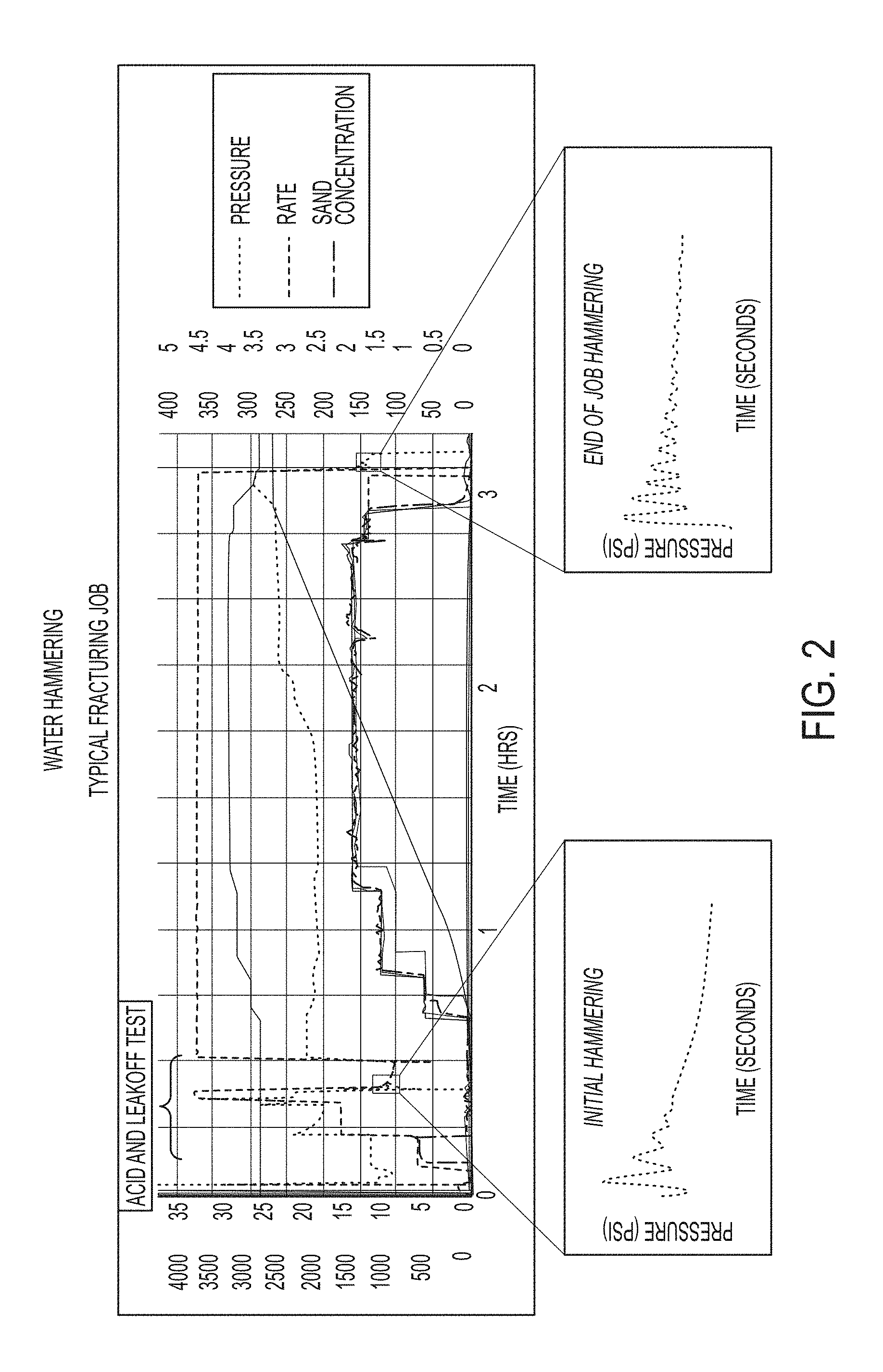
FIGS. 2 and 3 show an example of a fracturing treatment having a leak-off test performed at the beginning of the fracturing treatment, an initial water hammering effect of the leak-off test, and a final water hammering effect after the fracturing treatment;
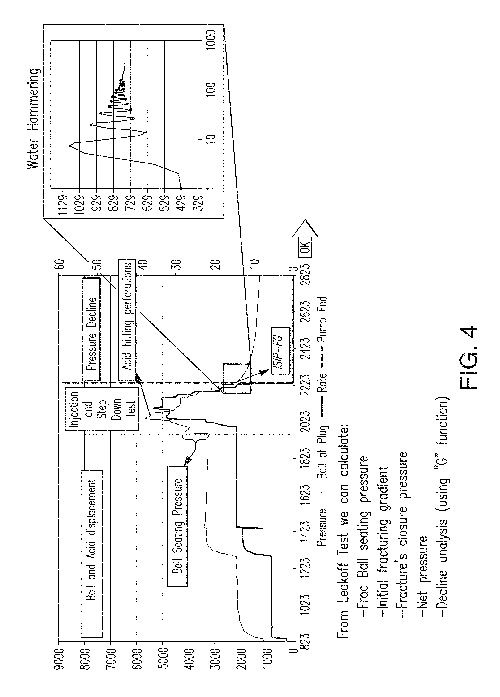
FIG. 4 is a closer or detailed view of the leak-off test shown in FIGS. 2 and 3;
FIG. 5 shows an example of measured pressure transient response;
FIG. 6 shows an example of multiple pressure transients generated during the pressure decline of the leakoff test;
FIG. 7 shows that the measured pressure transient response can identify a hydrocarbon-bearing reservoir quality;
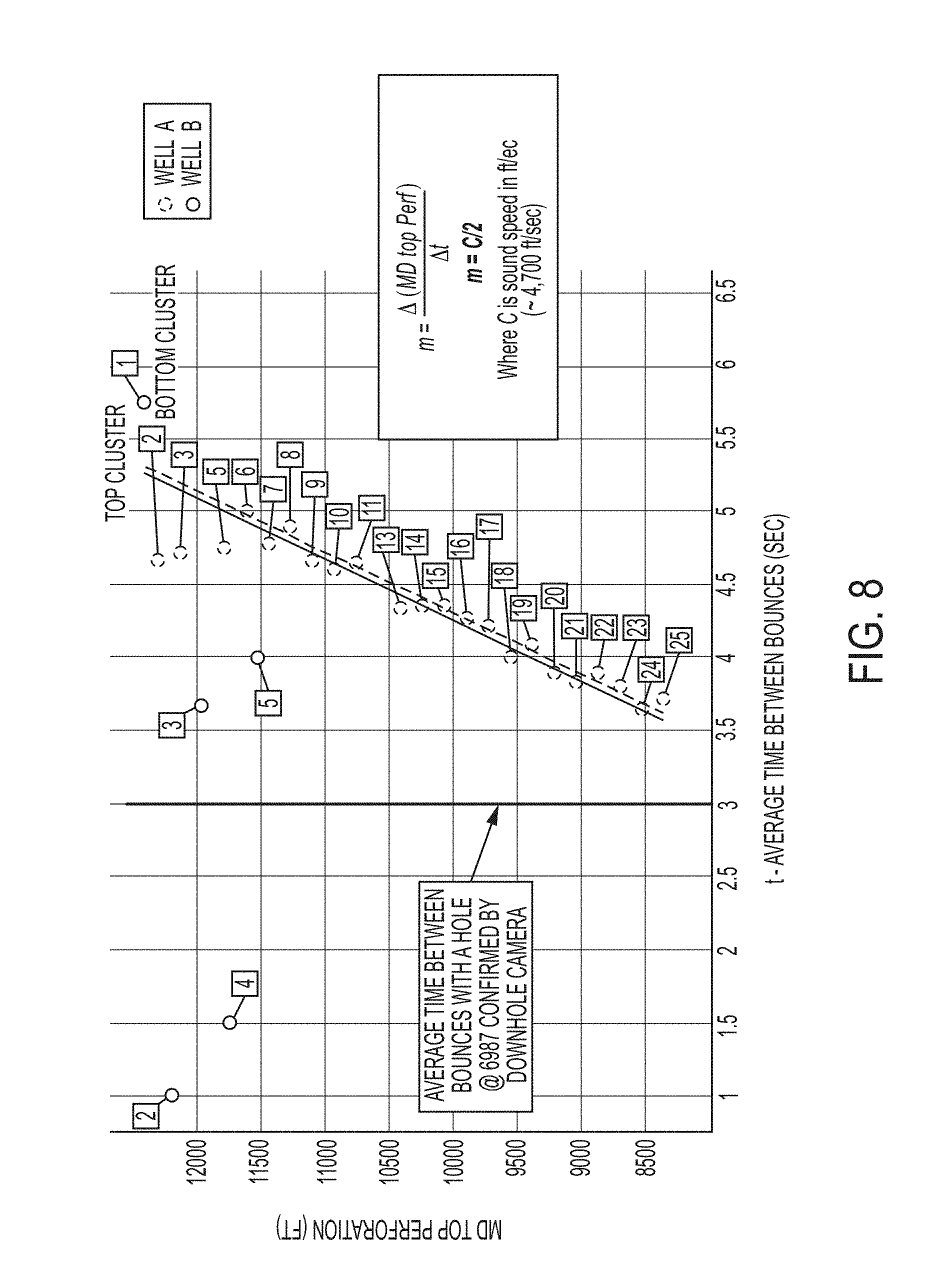
FIG. 8 shows at the measured pressure transient response can determine if there is a hole in the casing;
FIG. 9 shows a small section of an equivalent per unit length electrical model of a hydraulic wellbore/fracture system;
FIG. 10 shows matching between an electrical model response and an actual measured response for two different stages;
FIG. 11 shows the comparison of high Efficiency Coefficient and low Efficiency Coefficient;
FIG. 12 shows the comparison of high completions index and low completions index.
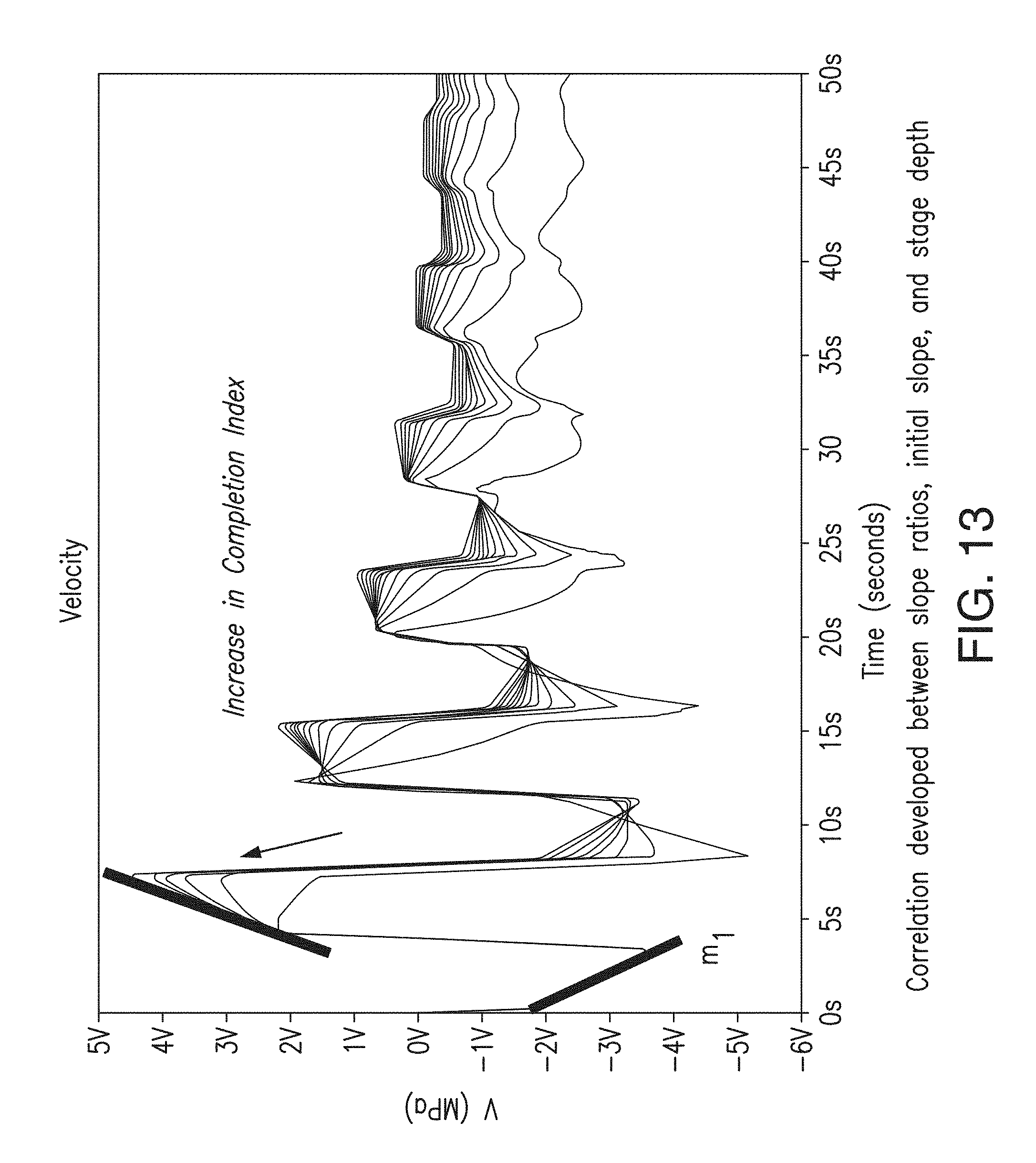
FIG. 13 shows the slope ratio variable for calculating the completions index and the correlation developed between slope ratios, initial slope and stage depth;
FIG. 14 shows how the completions index changes throughout a fracturing treatment;
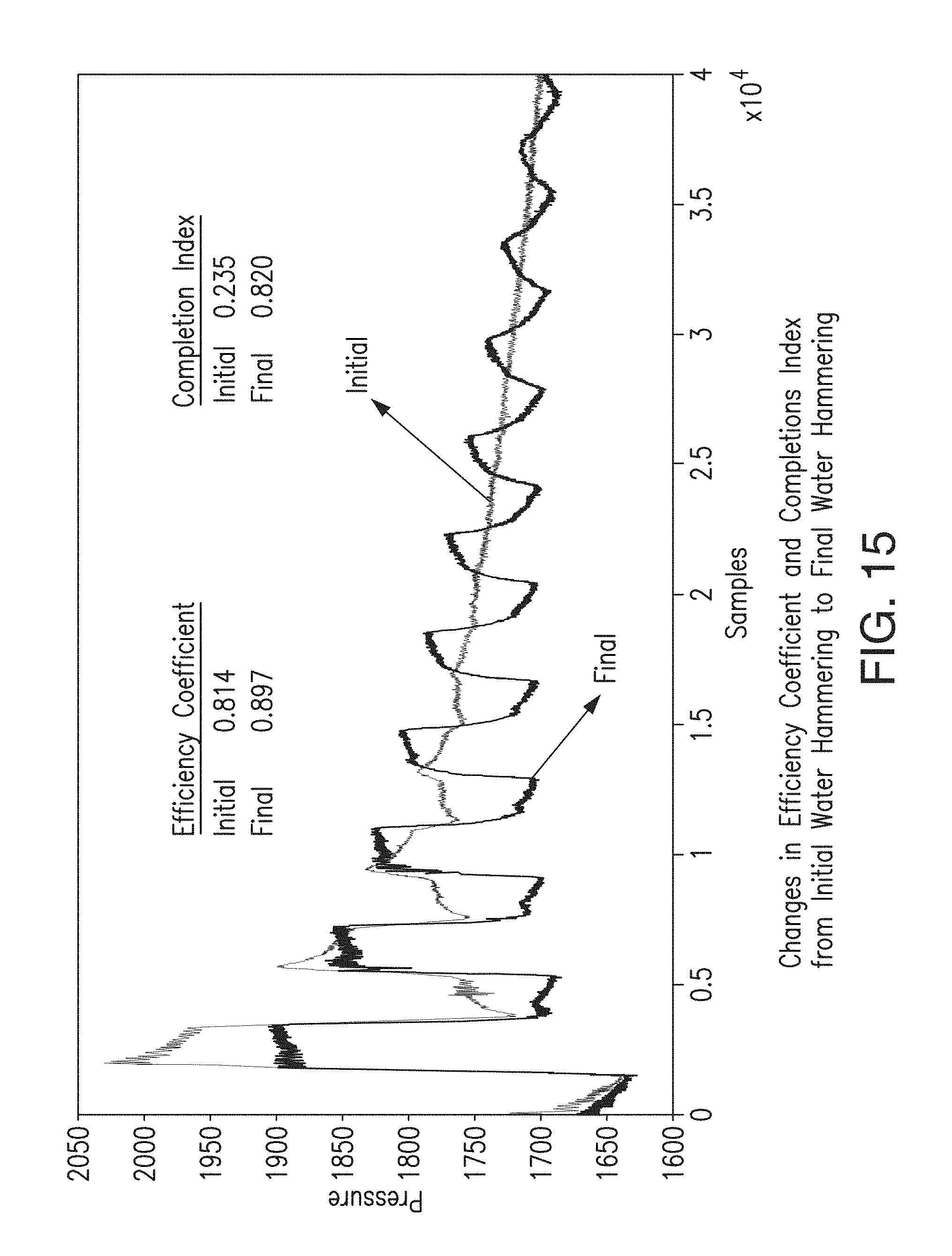
FIG. 15 shows changes in Efficiency Coefficient and completions index from initial water hammering to final water hammering;
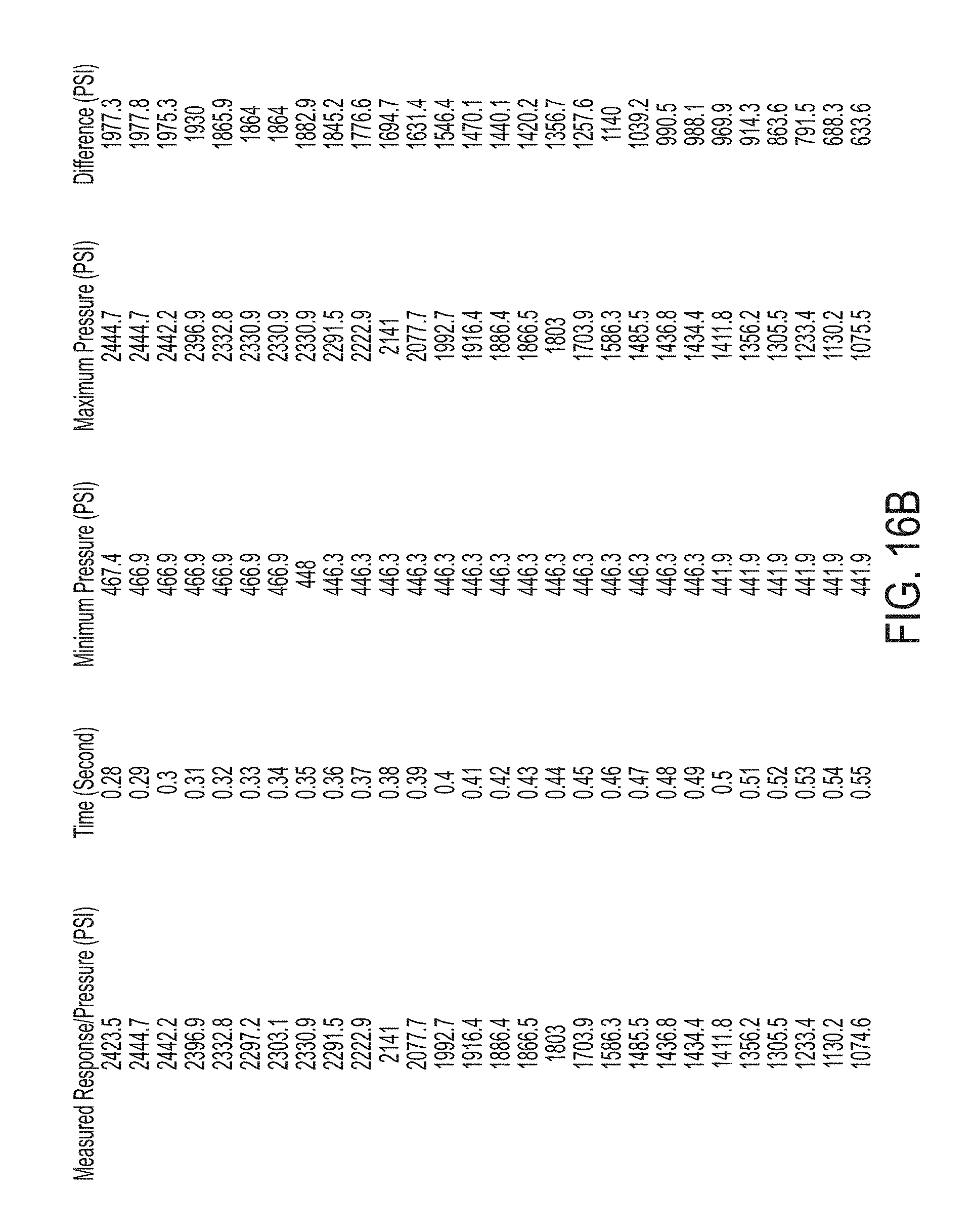
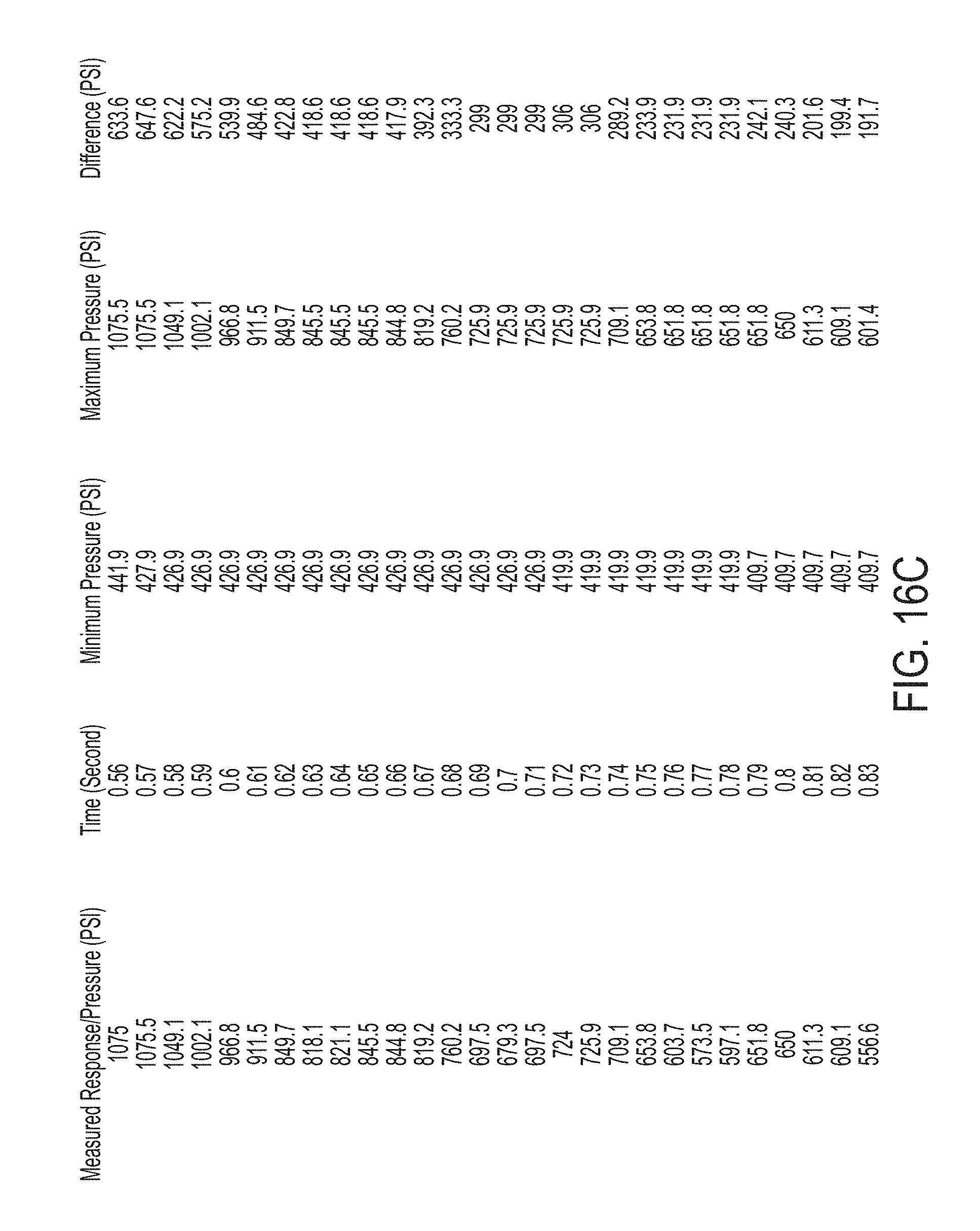
FIGS. 16A-16D show an example measured pressure transient response being transformed into a response having different pressure data;
FIG. 17 shows the graphical representations of the measured pressure transient response, the transformed response, and the decay curve of the transformed response; and
FIG. 18 shows an example correlation between reflection half-life and a modeled hydraulic resistance.
DETAILED DESCRIPTION OF THE INVENTION
Referring to FIG. 1, one embodiment of the method for determining a hydrocarbon-bearing reservoir quality 100 is illustrated. The method 100 comprises steps of performing a test determining a hydraulic pressure at which the reservoir will begin to fracture 110, generating a pressure transient during the test 120, measuring response of the pressure transient 130, determining fracture hydraulic parameters using the measured response 140, and optimizing a stimulation treatment to the hydrocarbon-bearing reservoir based on the determined fracture hydraulic parameters 150.
The step of performing a test determining a hydraulic pressure at which the reservoir will begin to fracture, or a leak-off test, 110 involves pumping a fluid, for example a hydraulic fracturing fluid, into a wellbore using a pressure pumping equipment. The wellbore extends from a surface to a reservoir and has one or more perforations extending through the production casing in communication with the reservoir. The pressure pumping equipment may be any equipment that is capable of pumping the fracturing fluid at a pressure into the wellbore. In addition to determining the hydraulic pressure at which the reservoir will begin to fracture, the leak-off test can also determine if the perforations are sufficiently open to establish communication with the reservoir. From the leak-off test, the ball seating pressure, the fracturing gradient (FG) of the formation, and the fracture closure time can be determined. A leak-off test is illustrated in FIGS. 2 and 3.
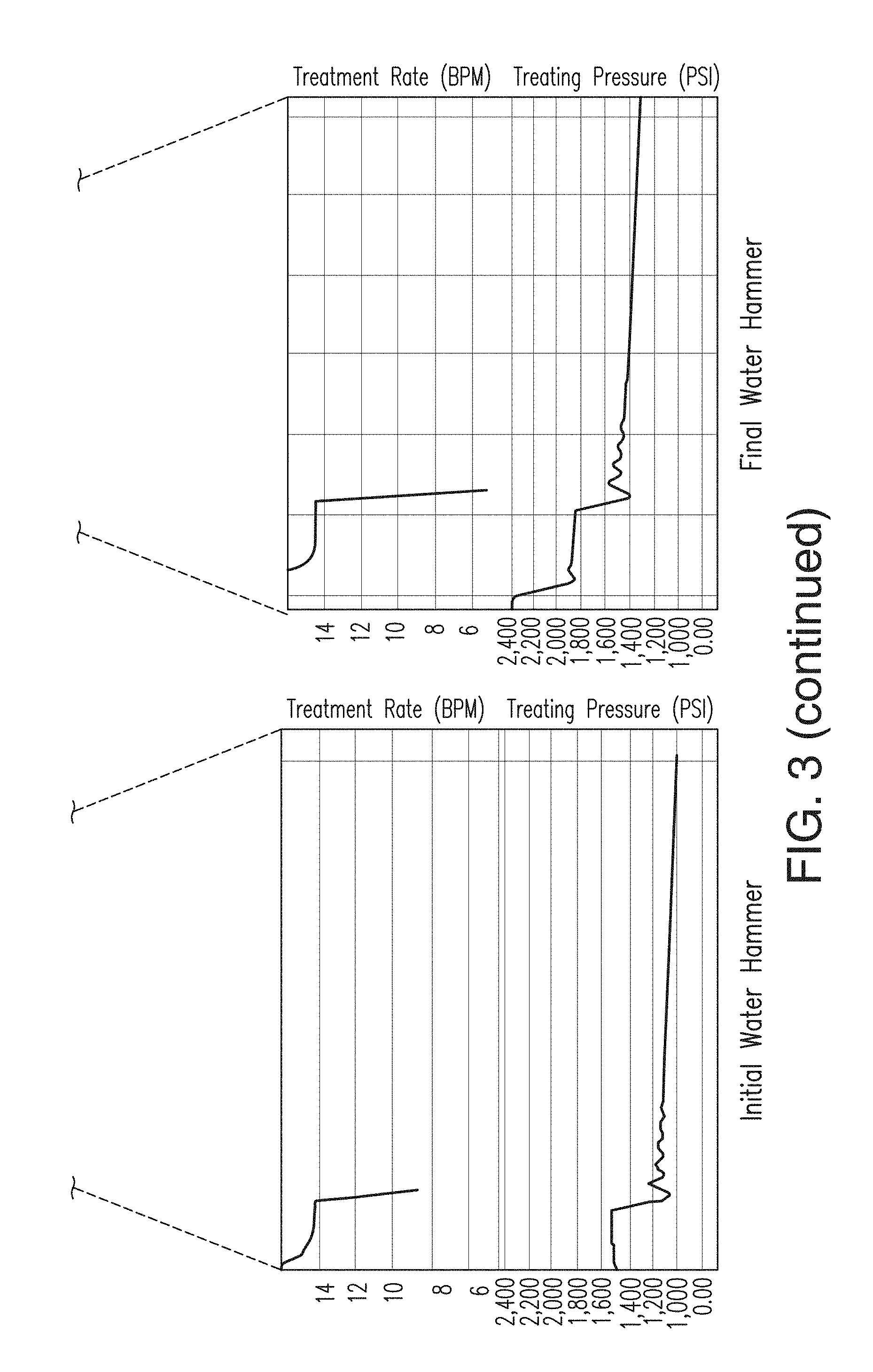
FIGS. 2 and 3 show an example of a fracturing treatment having a leak-off test performed at the beginning of the fracturing treatment, an initial water hammering effect of the leak-off test, and a final water hammering effect after the fracturing treatment. Referring to FIG. 2, the fracturing treatment in which the leak-off test is performed has a duration of approximately three hours from start to finish. FIG. 3 is a breakdown of FIG. 2 that shows the treatment rate (the top graph), the treatment pressure (the middle graph), and the proppant concentration (the bottom graph) of the fracturing treatment. The treatment rate in this example is approximately 32 barrels per minute between about 0.45 hour and 3.15 hour. The treating pressure is between 2,000 and 3,000 PSI from about 0.45 hour to 3.15 hour. The proppant concentration is between 0.5 and 1 pound per gallon (PPA) from about 0.6 hour to 0.9 hour, and between 1.5 and 2 PPA from about 0.9 hour to 3 hour. The leak-off test is labeled as the "acid and leak-off test" in FIG. 2 or the graph prior to the "rise" or "step" at approximately 0.45 hour in the treatment rate and the treatment pressure graphs. The leak-off test is initiated and concluded within approximately 30 minutes, or at about 0.5 hour, from the start of the fracturing treatment. After the leak-off test, and for the remaining two and half hours, water with chemicals is pumping into the wellbore and proppant is slowly added into the water to inject the stimulation fluid into the fractures in the reservoir.
Near the end of the leak-off test, a response or water hammering effect can be measured by generating a pressure transient and monitoring how the pressure transient declines with time. The very first 15 to 30 seconds after generating the pressure transient shows a lot of noise when the pressure transient is measured under low sampling frequency, such as 1 Hz, and that is the water hammering effect of the pressure transient. The pressure transient propagates to the perforations, reflects back to the surface, and travels in this manner back and forth until it attenuates completely. This response is shown as the initial water hammering graph in FIGS. 2 and 3. The same response may also be measured at the end of the fracturing treatment and is shown as the final water hammering graph in the same figures. The final water hammering graph shows more response or bounces because the fractures in the reservoir have been opened.
FIG. 4 is a closer or detailed view of the leak-off test shown in FIGS. 2 and 3. When the water hammering effect is measured at sufficiently high sampling frequency, such as sampling frequencies higher than 2 Hz up to 500 Hz, more water hammering effect can be seen from the measurement as shown in the plot labeled as "Water Hammering." The shape of the water hammering effect signal is directly depending upon the type of rock in the reservoir in communication with the perforations and is an indication of the rock quality. Therefore, when the water hammering effect signal is showing a good shape, i.e., more fluctuations and slower attenuation, the oil company can pump in more stimulation fluid in that stage to extract more oil and gas. If the water hammering effect is showing a had signal, i.e., less fluctuations and faster attenuation, the oil company can skip that stage or reduce the treatment size for that stage saving thousands of dollars in fracturing treatment and move onto the next stage. As such, the present invention provides real-time knowledge about the rock quality that can vary in each stimulation treatment stage of horizontal wellbores before the stimulation treatment is performed. By understanding the water hammering effect signal in each stage, oil companies can know when to pump more and when the pump less of the stimulation treatment.
A leak off test, which is also known as mini-frac, is a pumping sequence aimed to establish a hydraulic fracture, to understand, among other things, what is the pressure required to propagate a hydraulic fracture, and to estimate the minimum pressure at which the hydraulic fracture closes. A critical component of the test is the pressure monitoring after pumps as shut-down, which is commonly known as leakoff period or pressure fall off. During this period, fluid inside the open hydraulic fracture will leak off into the formation, continues until this process reaches a point that all fluid is leaked off and the hydraulic fracture closes. Another component of the test is the "step rate test," whereby the rate of fluid is gradually increased at the beginning of the test until a fracture is established or reaches the fracturing extension pressure and is reduced in a step down fashion at the end of the test. This test allows engineers to calculate the total pressure loss in between the rate steps so that the total number of perforations hydraulically connected to the fracture can be calculated. After the pumps are shut down, pressure is monitored for some time to determine fracture hydraulic parameters such as fracture closure pressure, presence of natural fractures, and leakoff coefficient for the fluid. Pressure may be monitored from several minutes to several hours and the fracture hydraulic parameters may be determined by using a "G" function.
Referring back to FIG. 1, the step of generating a pressure transient 120, the pressure transient is preferably generated by stopping or substantially reducing the pump rate of the pressure pumping equipment. But optionally, the pressure transient can be introduced by other methods that generate a pressure wave from the change of the inertia of the fluid, such as rapidly opening and closing a valve on the injection well head, or by other devices, such as a pressure oscillator or a mechanical shutter. The pressure transient travels from the surface to the reservoir through the perforations and reflects back to the surface after contacting the reservoir at the speed of sound in the wellbore fluid (normally water). Preferably, the pressure transient is generated within the first 15 to 30 seconds of the test determining a hydraulic pressure at which the reservoir will begin to fracture. After the pressure transient attenuates, additional pressure transients can be generated if desired (during the leak off test).
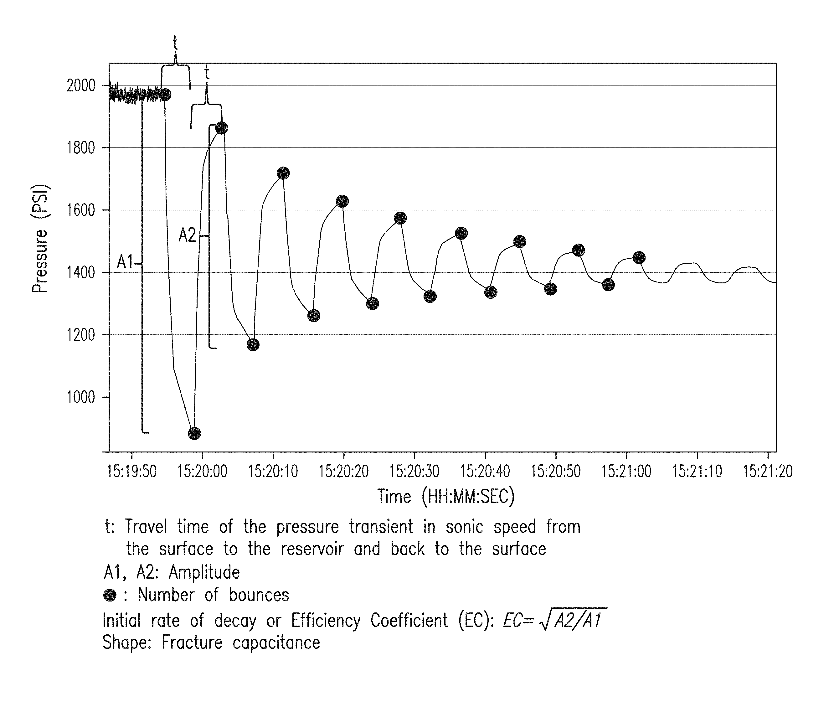
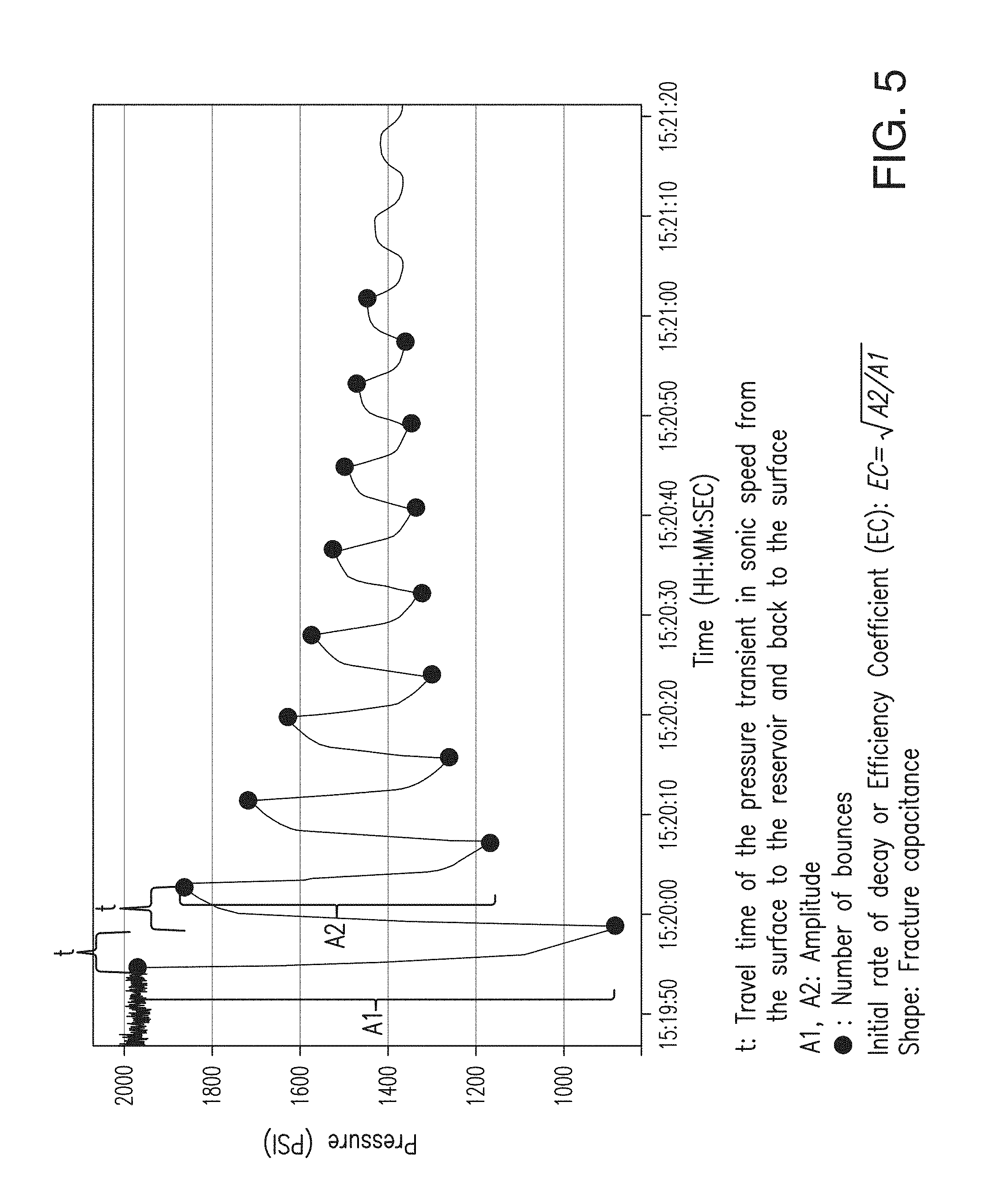
The response of the pressure transient, or the reflected pressure transient, is measured at sufficiently high sampling frequency such as at least 5 Hz. Alternatively, sample frequencies higher than 2 Hz up to 500 Hz may be used. The response is measured by a pressure transducer. An example of the measured response in high sampling frequency is shown in FIG. 5. The measured response is presented in a pressure-time plot. This measured response is also known as the water hammering effect. The y-axis is the pressure in pounds per square inch (PSI) and the x-axis is the time in minutes. The rounded dot represents the number of bounces from the surface. "t" represents the travel time of the pressure transient in sonic speed from the surface to the reservoir and then back to the surface through the wellbore fluid, which is the time between a peak and a trough on the plot. Such information can also be used to determine the distance of the perforations from the surface since the time between bounces is directly related to the distance to the perforations. A1 represents the initial decreasing amplitude of the waveform and A2 represents the next decreasing amplitude. A1 generally has a larger amplitude than A2. Based on A1 and A2, the initial rate of decay, or Efficiency Coefficient (EC), can be calculated by the following equation: EC= {square root over (A2/A1)}
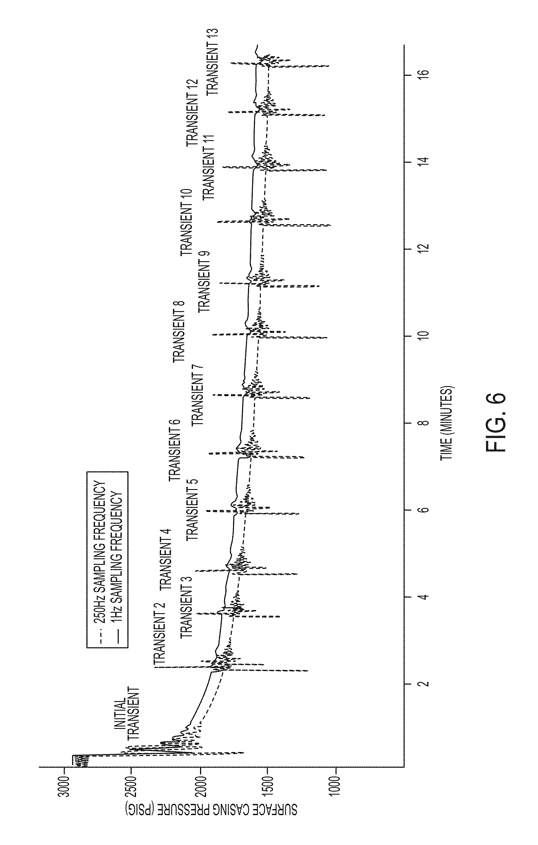
Although FIG. 5 shows that A1 and A2 are the preferred amplitudes, any two successive decreasing amplitudes may also be used. With the measured response in FIG. 5, fracture hydraulic parameters such as fracture closure pressure, fracture closure time, presence of natural fractures, and resistance of the perforations can be determined. Additionally, the shape of the waveform, which is determined by the combination of t, amplitudes, slopes on the waveform from the ISP (Instantaneous Shut-in Pressure) up to the A2 amplitude, can be used to calculate the fracture capacitance of the reservoir. While FIG. 5 shows only one pressure transient response, multiple pressure transients can be generated in each stimulation stage to obtain multiple responses for determining closure of the fractures in the reservoir. This determination is based on the comparison of the multiple responses with each other or the comparison of the most recently obtained response (or the most recently obtained flow resistance and fracture capacitance, which are described below) with a prior obtained response (or prior obtained flow resistance and fracturing capacitance). FIG. 6 shows an example of thirteen (13) pressure transients generated during the pressure decline of the leakoff test. The closure of the fractures can be observed from the reduction of the Efficiency Coefficient of each pressure transient versus time (or until the Efficiency Coefficient and fracture capacitance of each pressure transient no longer change with time). The figure shows responses measured at 1 Hz and 250 Hz sampling frequencies. Responses showing inconspicuous fluctuations correspond to measurement at 1 Hz sampling frequency and responses showing pronounced fluctuations correspond to measurement at 250 Hz sampling frequency.
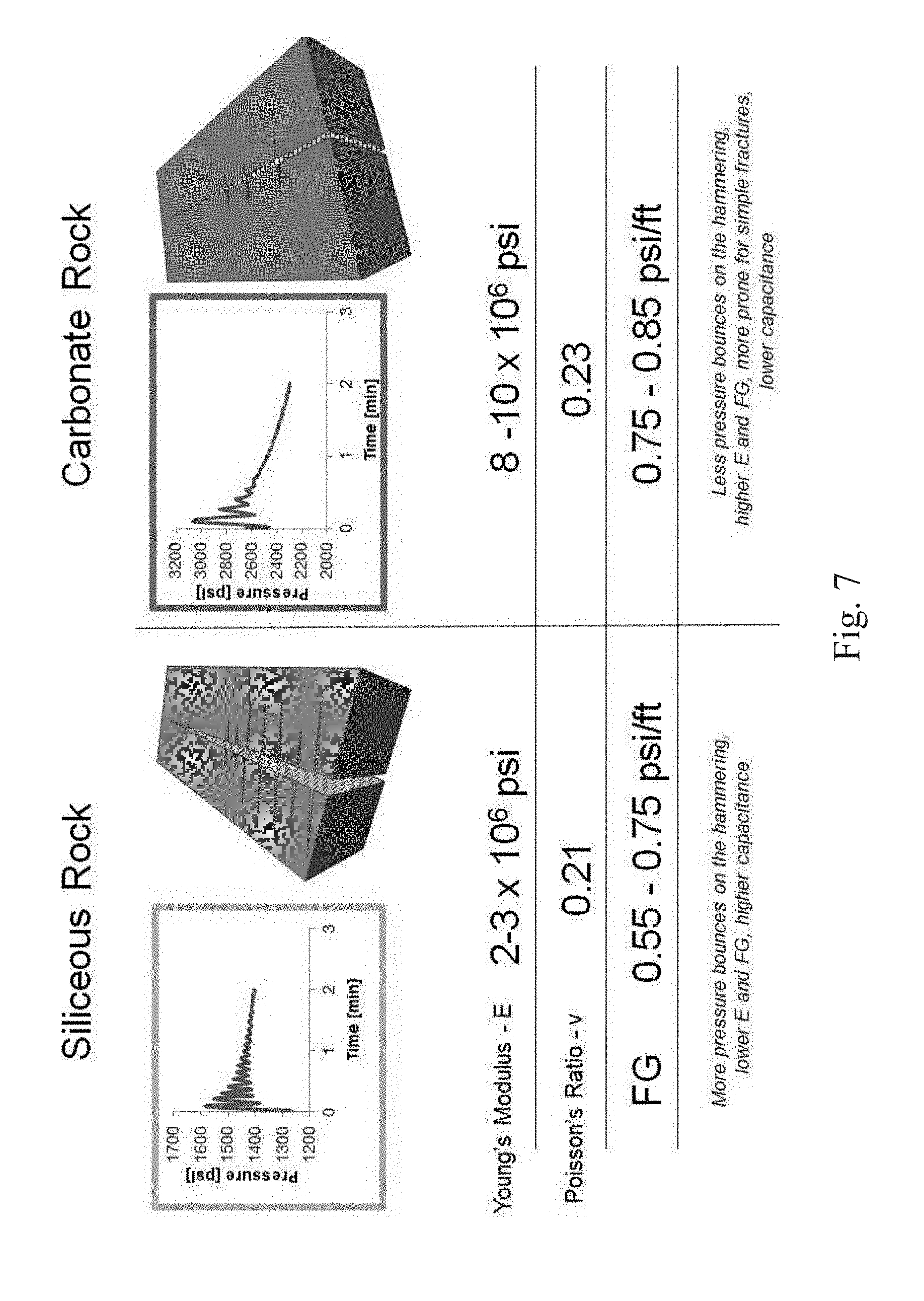
The measured response can identify reservoir quality. Measured responses show significant differences for different reservoirs or rocks having similar wellbores (for example, multiple wells in a given field), as the pressure transient travels outside the wellbore through the perforations of the wellbore and into the adjacent formation/rocks. If the transient pressure did not travel outside the wellbore, the expected responses would be similar for comparable wellbores. This also proves that the perforations are open and in communication with the formation. This identification ability is shown in FIG. 7. On the left of FIG. 7, a siliceous rich mud rock (shale), which has a lower Young's modulus and a lower fracturing gradient, produces a lot of fluctuations or hammering (higher capacitance). On the right of FIG. 7, a carbonate rich mud rock (shale), which has a higher Young's modulus and a higher fracturing gradient, produces a lot less hammering (lower capacitance Thus, based the amount of hammering, one can obtain an initial impression of whether the rocks are prone to simple or complex fracturing.
The measured response can also be used to determine if there is a hole in the casing. Referring to FIG. 8, two wells A and B are plotted. Well A is represented by lighter-colored dots whereas Well B is represented by darker-colored dots. Well A has a casing without any holes and its plot shows a pattern close to a linear line for the various stages where pressure transients were measured. The slope m of the linear line may be determined by the following equation:
.DELTA..function..times..times..times..times..DELTA..times..times. ##EQU00001##
MD top perforation is the measured depth to the top perforation. The slope m is measuring the change in measured distance to the top perforation for successive stages in the well divided by the change in time. The slope m may also be determined by dividing the speed of sound C by 2.
Well B, on the other hand, has a casing with a hole and its dots spread everywhere on the chart without a general pattern. Based on the measured response, it was confirmed by a downhole camera ran on this well that a hole was located in the casing at a measured depth of 6987 feet.
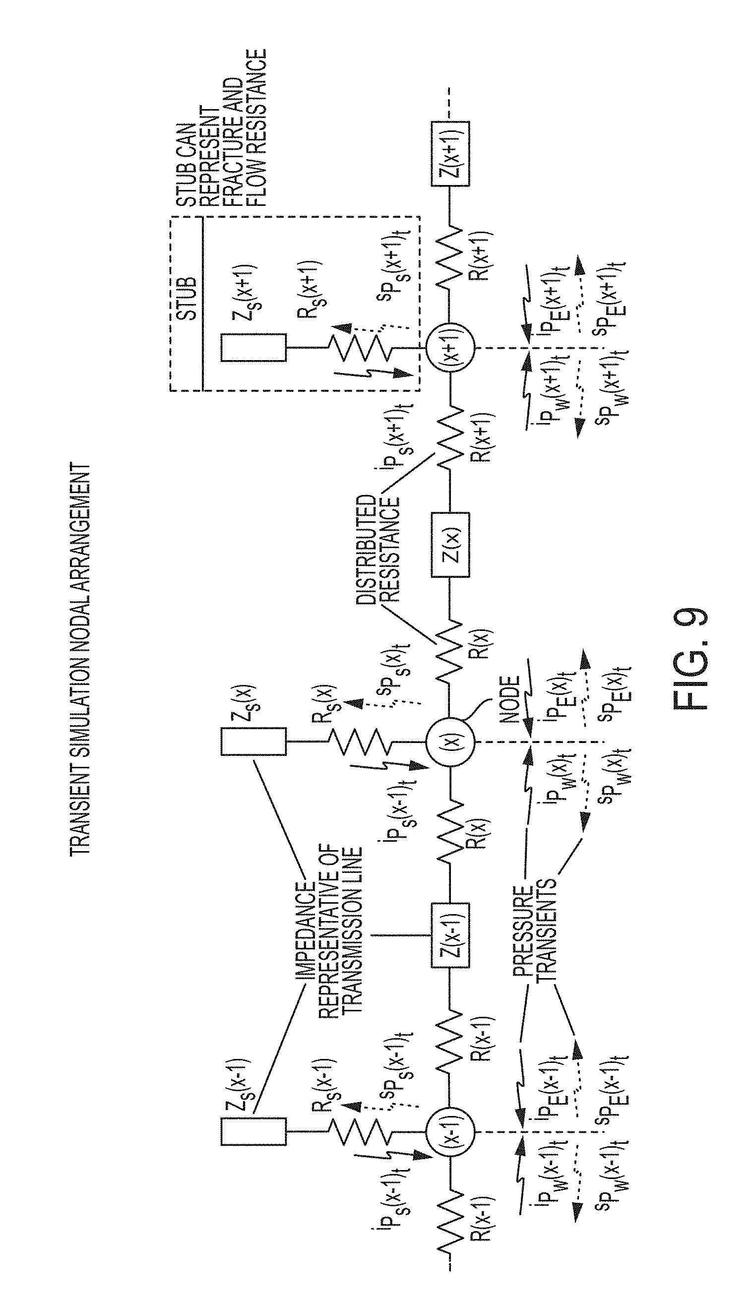
For every hydraulic wellbore/fracture model, there is an equivalent electrical model. The wellbore or casing may be modeled as a lossy transmission line using resistors, capacitors, and inductors. The values of all these electrical components are known if one knows the depth of the well, the size of the casing, and the temperature and type of the fluid used in the well. Some or all of these values may be lumped into an impedance representing the electrical property or mechanical property of the wellbore. The generated pressure transient inside the casing may be modeled as an input voltage on the transmission line. The perforations of the casing, which provide communication to the reservoir, may be modeled as a resistor. If the perforations are small, the resistance is high and vice versa. The reservoir itself or the quality of the reservoir may be modeled as a capacitor.
FIG. 9 represents a small section of an equivalent per unit length electrical model. This small section of the electrical model corresponds to a small section of the horizontal portion of the wellbore. This small section of the electrical model is divided into three (3) nodes ((x-1), (x), and (x+1)) and each node is associated with a stub that is spaced along the horizontal portion of the wellbore for example, every 30 feet. The stub associated with each node is used to represent an area of the reservoir and any changes in casing properties, otherwise the impedance of the stub, Zs, is set sufficiently high such that no current flows into the stub. A simulated response similar to the actual measured response can be obtained from each node by generating an input voltage, or simulated pressure transient, to the electrical model or circuit. A stub modeling a fracture, for instance, Zs(x+1) and Rs(x+1), represents fracture capacitance Zs(x+1) and flow resistance Rs(x+1). Each impedance, Zs(x-1), Zs(x), Zs(x+1), Z(x-1), Z(x), or Z(x+1), has an inductive component and a capacitive component and they are configured to be the equivalent circuit of a transmission line (not shown). While fracture capacitance appears to be impedance, or Zs, in the figure, the value of the impedance is essentially capacitance. When the electrical model in FIG. 9 is simulated, the inductive component of Zs is treated as if it has little to no inductance, and therefore, the impedance becomes a capacitor representing an area of the reservoir or the fractures in that area of the reservoir. In other words, the electrical model by default presents or sees an area of the reservoir or the fractures in that area of the reservoir as impedance but the value of the impedance is simulated to be based on a capacitor. Although this figure shows only three nodes, there can be more nodes as this figure represents only a small section of the electrical model or the horizontal portion of the wellbore. The distance between two adjacent nodes typically can range from 10 to 250 feet. Other ranges are also possible depending on the scale of the hydraulic wellbore system.
R(x-1), Z(x-1), and R(x) (and R(x), Z(x), and R(x+1), etc) are lumped impedance representative of a transmission line (Z(x-1)) and resistance (R(x-1) and R(x)) values and they represent a lateral portion of the casing connecting adjacent nodes or adjacent areas of the reservoir. All these values are fixed and can be determined based on the depth of the well, the size of the casing, and the fluid in the casing.
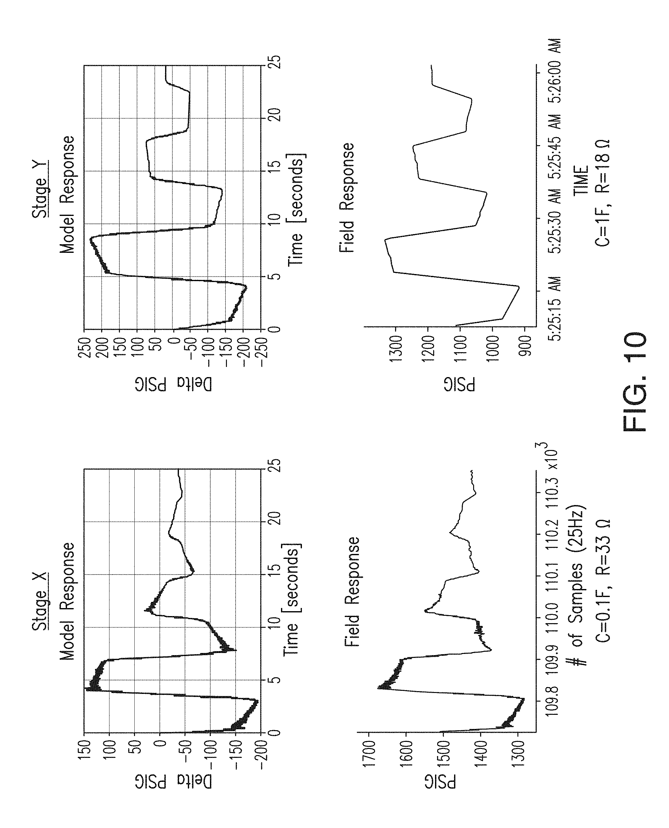
Therefore, by using an equivalent electrical model, one can obtain a simulated response similar to the actual measured response for each stage of the horizontal portion of the wellbore. A simulated response can be created to match the actual measured response by adjusting the resistor in the stub and the capacitor of the impedance component in the stub or by solving their resistance and capacitance through numerical optimization. Once the simulated response matches to the actual measured response, the obtained resistance is known as the flow resistance and the obtained capacitance is known as the fracture capacitance. FIG. 10 shows such matching for two different stages. At stage X, the simulated response (the top graph) matches to the actual measured response (the bottom graph) when the resistance is 33 ohm and the capacitance is 0.1 farad. At stage Y, the simulated response matches to the actual measured response when the resistance is 18 ohm and the capacitance is 1 farad.
Thus, by using an electrical model, simulated responses with their associated flow resistances and fracture capacitances can be obtained for previous actual fracture stimulation operations, future actual stimulation operations, and any other stimulation operations that one may encounter since the information regarding the well, the casing, and the fluid are already known, will be known, or can be predicted in advance. All these simulated responses, flow resistances, and fracture capacitances may be saved in a database or lookup table for comparison with future stimulation operations. In one embodiment, the comparison may be performed by adjusting the resistor in the electrical model first to determine the flow resistance and then adjusting the capacitor to determine the fracture capacitance. Therefore, it is possible to model every expected response and different combination of depth, fracture flow resistance, fracture capacitance, and response at the surface in terms of the pressure transient that is generated at the surface for a given field. The benefit is that hydraulic properties of the fracture system of the reservoir can be inferred by just looking at the pressure responses observed at the surface during the water hammering. The model allows one to infer the flow resistance and the hydraulic capacitance of the fracture based on the pressure response measured at the surface. In other words, if the comparison shows a match, the flow resistance and fracture capacitance of the actual fracture stimulation operation can be obtained from the flow resistance and fracture capacitance of the matched simulated response. With this lookup table, one does not need to manually change the resistance and capacitance in the electrical model for matching its simulated response to every measured response. The benefit of having the lookup table or database allows an operator to calculate these parameters very quickly. The operator can get the transient response from the initial injection or leak off test before the primary stimulation of every stage in a horizontal wellbore, thereby providing the operator valuable information needed on a near real time basis to optimize each particular stage before pumping any proppant.
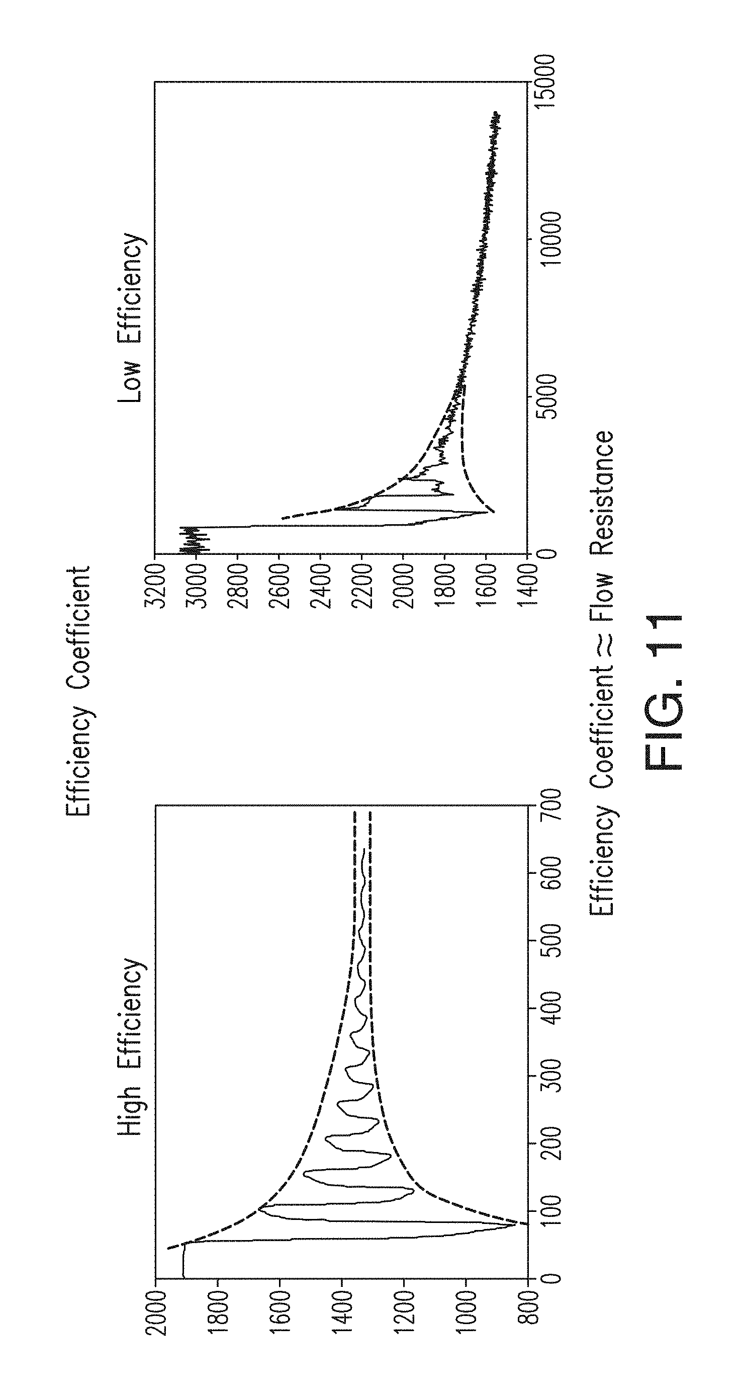
The flow resistance can also be approximated by the Efficiency Coefficient. The Efficiency Coefficient is determined by how fast the measured response decays (i.e., the initial rate of decay) and the number of bounces the measured response contains. These determining factors are directly related to the near wellbore flow resistance or the flow through the perforations. High Efficiency Coefficient means that the perforations are open and have less resistance, and low Efficiency Coefficient means that the perforations are narrow and have more resistance or that there is a tortuous path connecting the wellbore with the hydraulic fracture. This is shown in FIG. 11.
The fracture capacitance is also known as the completions index. This value is directly related to the slope (darkened line) of the simulated response as shown in FIG. 12, and it indicates whether the reservoir is a compliant or non-compliant system. Referring to FIG. 12, a positive slope is considered as high index and it indicates that the reservoir is a compliant system. A negative slope is considered as low index and it indicates that the reservoir is a non-compliant system. A compliant or non-compliant system provides information regarding how rigid the reservoir is. A compliant system means that the reservoir is less rigid (presence of natural fractures), the volume of a bounded fluid would expand rapidly with increase in pressure and contact more surface area inside the reservoir. A non-compliant system means that the reservoir is more rigid, the volume of a bounded fluid would remain relatively static with increase in pressure and contact less area inside the reservoir. Generally, a rock showing a compliant system is considered as good rock quality and is more ideal for a stimulation treatment. Conversely, a rocking showing a non-compliant system is considered as lower rock quality and is less ideal for a stimulation treatment. As such, when one obtains the completions index, or the value of the capacitance in the simulated response, quality information of the reservoir is also obtained.
In addition to obtaining the fracture capacitance by comparing the simulated responses to the measured response in the manner discussed above, one can also obtain the fracture capacitance through numerical optimization. One way of performing numerical optimization is via a neural network. In this invention, the neural network is a computational model configured to receive four variables extracted from the measured response, compares those variables to the same variables in the simulated responses, and calculates the completions index if the comparison matches. These four variables are the depth of the stimulation stage, the Efficiency Coefficient, the slope ratio, which is m1/m2 as shown in FIG. 13, and the initial pressure drop in the test of determining a hydraulic pressure at which the reservoir will begin to fracture. FIG. 13 also shows the correlation developed between slope ratios, the initial slope, and the stage depth. The neural network compares the variables and calculates the completions index based on training weights obtained from simulations and previous measurements (optimizing a numerical model to match the measured response). During this optimization, the Efficiency Coefficient and the completions index are optimized together or simultaneously. The optimization of the Efficiency Coefficient simultaneously optimizes the completions index and vice versa. The neural network may also be utilized to determine the fracture capacitance by interpolation. The employment of a neural network provides speedy comparison and calculation of the completions index.
Another way of performing numerical optimization to obtain the fracture capacitance is via, numerical simulation of the electrical model in FIG. 9. One can use numerical optimization to match the electrical model output to find a best fit to the measured field data. Using the equivalent per unit length electrical model shown in FIG. 9, one can determine the correct flow resistance and completions index in order to match the observed field response. These values are found through a process of numerical optimization, wherein a numerical simulator solves many iterations of the electrical model output with varying flow resistance and completions index values. Each iteration is assigned a fitness or a numerical value corresponding to the quality of the match to the measured field response. The numerical simulator then outputs the values of the flow resistance and completion index with the best fitness values. Like the numerical optimization based on a neural network, the flow resistance and fracture capacitance are also optimized together or simultaneously. The optimization of the flow resistance simultaneously optimizes the fracture capacitance and vice versa.
Therefore, referring to the step of determining fracture hydraulic parameters using the measured response 140 in FIG. 1, one can determine flow resistance and fracture capacitance by either comparing the simulated response to the measured response with help from a lookup table or employing numerical optimization. Based on the determined flow resistance and fracture capacitance, one can optimize a stimulation treatment to the reservoir 150. The stimulation treatment may be a hydraulic fracturing treatment. The optimization of the stimulation treatment may be adjusting the volume, properties or rate (i.e., number of barrels per minute) of the fracturing fluid is required to fracture the reservoir, adjusting the volume, size or type of proppant carried by the fracturing fluid, or omitting a hydraulic fracturing treatment altogether for a given stage.
FIG. 14 shows how the completions index changes throughout a fracturing treatment. In this example, the fracturing treatment is divided into three phases instead of one single continuous fracturing treatment to better observe capacitance change and to adjust stimulation fluid accordingly. Before any treatment is performed, the reservoir initially has a completions index of 0.03. After the first phase of the fracturing treatment is performed by pumping stimulation fluid with 92,000 lbs. of sand and the pumping is shut down, which corresponds to the step of the pressure waveform to the left most of the plot, the completions index or capacitance rises quickly to 0.087. This change in capacitance is an indication of the rock quality and can be used to optimize the fracturing treatment for a particular stage. The subsequent phases of the fracturing treatment show that increasing the amount of proppant yields minor increase in capacitance. As such, an operator knows how rigid the rock is and the optimal amount of proppant to fracture the rock in this particular stage. Based on this figure, the operator may not want to add any more proppant into the fluid after the second phase or after the third phase since the completions index would not change much and the cost of fracturing treatment can be reduced. By analyzing the completions index to determine reservoir quality, the method is also known as Completions Index Analysis.
While FIG. 14 shows that the method of the present invention is conducted during a fracturing treatment, the method may also be performed after the fracturing treatment to provide indications on the quality of the fracturing treatment just performed.
Based on the foregoing, using the measured responses from the water hammering effect allows an operator to see the variations in the rock quality so one can recognize the good pan of the lateral (i.e., horizontal wellbore) and what is the poor part of the lateral. Knowing this information, the operator can make near real time decisions to optimize the stimulation treatments of the various stages of a wellbore. Thus, an operator can determine which sections of the wellbore may justify an even larger treatment than was originally planned and which sections could be omitted, thereby reducing the overall cost of the treatment and/or improving the effectiveness of the treatment.
FIG. 15 shows a comparison of the initial water hammering effect and the final water hammering effect for a stimulation stage based on the Efficiency Coefficient and the completions index. The initial water hammering effect is the effect measured prior a fracture treatment whereas the final water hammering effect is the effect measured after the fracture treatment. Both have similar input slopes or utilize similar pressure transients. The final water hammering effect shows that the signal decays much slower after the fracture treatment, which indicates that the fracturing fluid and the perforations have a better connection to the reservoir. The fracture treatment has eroded the tortuous path of the fractures and it becomes easier to establish a communication from the wellbore to the reservoir. As such, both the Efficiency Coefficient and the completions index are higher after the fracture treatment. The Efficiency Coefficient before and after the fracture treatment are 0.814 and 0.897, respectively. The completions index before and after the fracture treatment are 0.235 and 0.820, respectively.
As discussed above, the flow resistance can be determined by the rate of decay of the measured pressure transient response and the rate of decay can be calculated from two successive decreasing amplitudes. Alternatively, the rate of decay can be calculated by transforming the measured pressure transient response to produce a transformed response and calculating the rate of decay of the transformed response. The measured pressure transient response or simply the measured response) provides pressure information over a period of time. The transformed response provides pressure information different from that of the measured response over the same period of time (e.g., different pressure behavior over the same period of time).
In one embodiment, the measured response may be transformed by generating a window defining a period of time over the measured response, determining the maximum pressure and the minimum pressure in the period of time defined by the window, calculating the difference between the maximum pressure and the minimum pressure, and producing the difference as a data point of the transformed response. The window may define a period of time such as 0.5 second, 1 second, 2 seconds, or any other duration. The measured response may have pressure data measured at a frequency. The frequency may be 0.005, 0.008 second, 0.01 second, 0.05 second, or any other frequency. Preferably, the window has a duration of 1 second and a frequency of 0.01 second. Within the time duration of the window, there are a number of pressure measurements in the measured response with each measured at the specified frequency, and the maximum pressure and the minimum pressure are determined from those pressure measurements. The difference between the maximum pressure and the minimum pressure is a data point of the transformed response, and it corresponds to the first data point of the measured response in the window or the data point of the measured response that is first in time in the window. The determination of the maximum pressure and the minimum pressure and the calculation of the difference starts from the beginning of the measured response or 0 second. A data point refers to a measurement at a specific time whereas data refers two or more measurements or all the measurements collectively.
The window may slide on the measured response at an increment of time to determine the maximum pressure and the minimum pressure in the period of time defined by the slided window and to calculate the difference between the maximum pressure and the minimum pressure in the slided window. The window slides without changing its time duration (e.g., the time duration of the window is the same before and after sliding). The increment of time and the frequency may be the same (e.g., 0.01 second). The determination of the maximum pressure and the minimum pressure and the calculation of their difference in the slided window involve the same computations as those discussed above. The window may continue to slide, determine the respective maximum pressure and the respective minimum pressure, and calculate the respective difference for the entire measured response. The differences collectively create the transformed response with each difference being a data point of the transformed response.
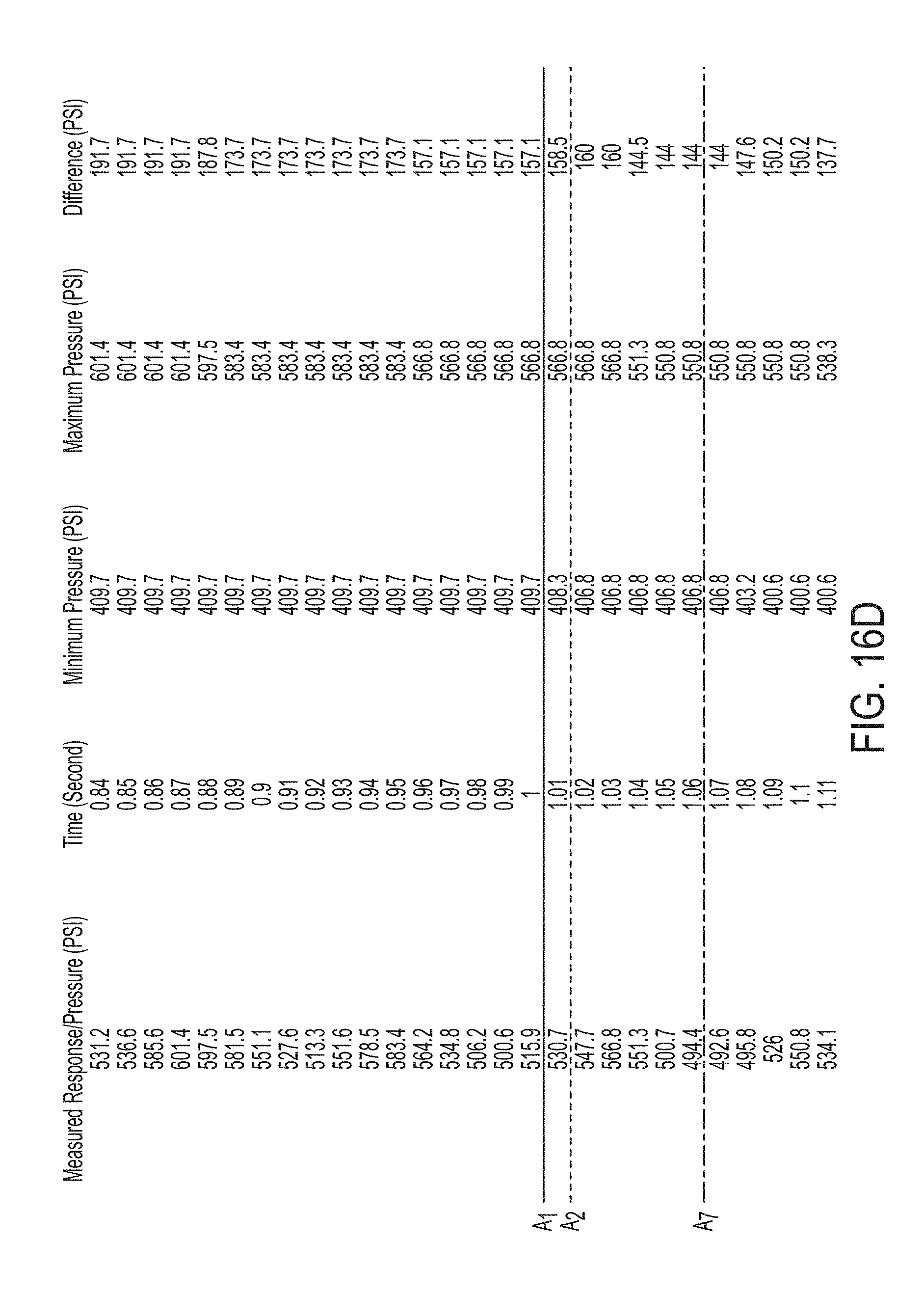
FIGS. 16A-16D show pressure data of an example measured response 1605 and pressure data of an example transformed response 1610. In these Figures, the transformed response 1610 (or the differences) is obtained by using a window A having a 1 second duration and by sliding the window at an increment of 0.01 second over the measured response 1605. The measured response 1605 had the pressure measured at a frequency of 0.01 second. Given the length of the measured response and the frequency/increment used, only part of the measured response and part of the transformed response are shown (up to 1.11 second).
The measured response 1605 includes a number of measurements with each conducted at every 0.01 second starting from 0 second. The transformation starts from the beginning of the measured response and determines the maximum pressure and the minimum pressure in the 1-second duration of the window A (see FIGS. 16A and 16D). In that window, e.g., from 0 second to 1 second defined by window A.sub.1, the minimum pressure in the measured response 1605 is 500.6 PSI and the maximum pressure in the measured response 1605 is 2624.2 PSI. The difference between the two pressures is 2123.6 PSI. The difference corresponds to the first data point in the transformed response 1610 or the first data point (e.g., 2612.1 PSI) of the measured response 1605 in the window A.sub.1. The transformation then slides the window A by an increment of 0.01 second. In that window, e.g., from 0.01 second to 1.01 second defined by window A.sub.2, the minimum pressure in the measured response 1605 is still 500.6 PSI and the maximum pressure in the measured response 1605 is still 2624.2 PSI. Accordingly, the difference between the two pressures is also still 2123.6 PSI. The difference corresponds to the second data point in the transformed response 1610 or the first data point (e.g., 2563 PSI) of the measured response 1605 in the window or the slided window A.sub.2.
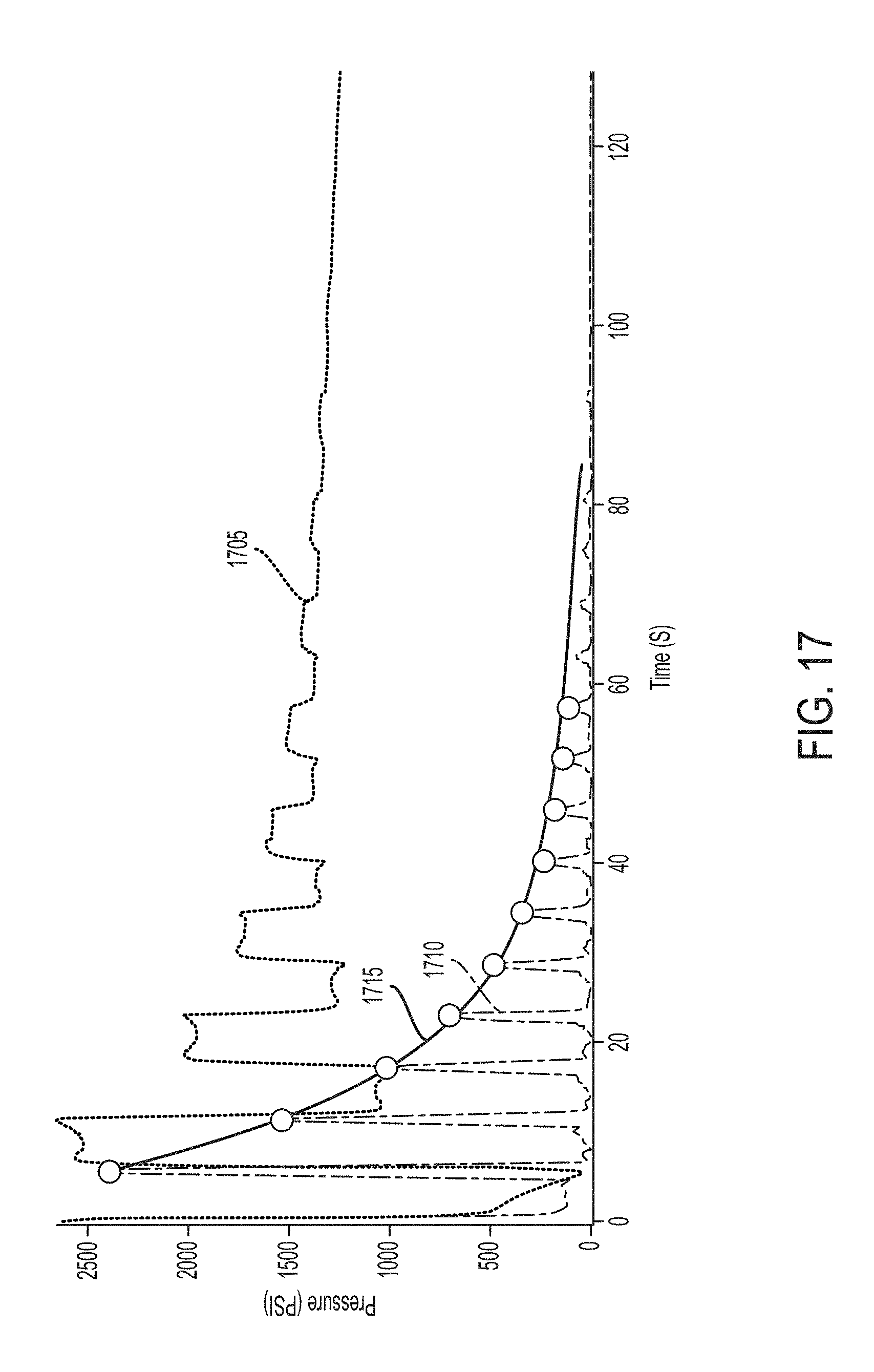
The transformation may continue to slide the window A at the specified increment. When the window A reaches to 0.06 second, which covers the measured response from 0.06 second to 1.06 second defined by window A.sub.7, the minimum pressure in the measured response 1605 is 494.4 PSI and the maximum pressure in the measured response 1605 is 2618.4 PSI. The difference between the two pressures is 2124 PSI. The difference corresponds to the seventh data point in the transformed response 1610 or the first data point (e.g., 2618.4 PSI) of the measured response 1605 in the window or the slided window A.sub.7. The transformation may continue to slide the window A until the entire measured response is transformed. The transformed response may be a response produced for the same period of time from which the measured response is obtained (e.g., if the measured response is obtained for 1.11 second, or from 0 to 1.11 second, then the transformed response is also obtained for that 1.11 second), but has a different pressure behavior in time (e.g., the response or the signal forms a different shape). The transformed response is a new time series curve. Each measurement in the measured response 1605 has a corresponding transformed data point. The transformation process may be known as a rolling max-min technique. FIG. 17 shows the graphical representations of the measured pressure transient response 1705 and the transformed response 1710.
Windows A.sub.1, A.sub.2, and A.sub.7 all refer to the same window having the same duration. The subscripted number is used merely to differentiate their positions on the measured response 1605.
The rate of decay of the transformed response 1710 is then determined. The rate of decay is determined by finding the peaks of the transformed response 1710 and fitting an exponential decay to the peaks to produce a decay curve 1715, which is also shown in FIG. 17. The exponential decay or the decay curve 1715 indicates how quickly in time the transformed response decays. This rate of decay is then used to calculate a reflection half-life or a parameter that measures flow resistance.
In particular, the rate of decay Y of the transformed response 1710 may be determined by an exponential function that has the following form: Y=Ae.sup.-Cx
where A is the initial quantity (i.e., the quantity at time t=0), C is the decay constant, and x is the number of cycles or reflections. The number of reflections is also the number of peaks in the transformed response 1710. The amplitude (or pressure) of each peak is selected and the plurality of amplitudes are graphed with respect to the number of peaks. The exponential decay is fitted to this function rather than to a function of time. The exponential decay is not fitted as a function of time because the depth of a given completion stage is going to drive the time required for the pressure transient to reach the perforations and reflect back to the surface, thereby increasing or decreasing the time between pulses of the measured response. After fitting the exponential decay, the number of peaks required for the amplitude of the transformed response 1710 to decay by one-half is calculated. The number of peaks can be calculated by solving x in the above equation when Y=1/2A. The solved x is the reflection half-life. The reflection half-life describes the decay characteristics for different water hammer responses. A higher reflection half-life indicates that the water hammer response (or the measured response) takes more reflections to decay and correlates to a lower hydraulic resistance. A lower reflection half-life indicates that the water hammer response decays more quickly and correlates to a higher hydraulic resistance.
The reflection half-life (solid line) can be correlated to a modeled hydraulic resistance (dotted lines) as shown in FIG. 18. The modeled hydraulic resistance is an element of the electrical model that is varied over a range to observe how it affects the rate of decay of the measured response. For example, the electrical model may be the model shown in FIG. 9 and the modeled hydraulic resistance may be determined by adjusting the resistor Rs(x-1), Rs(x), or Rs(x+1) over a range of values when the other valuables are known or fixed to obtain several responses. This resistance, for example Rs(x+1), can represent the hydraulic resistance at the casing to fracture system interface. This is also modeled at the depth of the perforations for a given completion. The other resistance values in FIG. 9 are used to capture the hydraulic impedance of the casing and are not varied for a fixed diameter casing. The reflection half-life can be correlated to those responses over a range of Rs(x+1). This correlation allows for the constraint of the numerical optimization or can be used directly to evaluate the flow resistance of the measured response. Hydraulic resistance also refers to the flow resistance of the perforations between the wellbore and the reservoir.
The transformation, the calculation of the decay rate, the calculation of the reflection half-life/parameter, and the correlation between the reflection half-life/parameter and the modeled hydraulic resistance can be performed by a processor (e.g., CPU) or a specialized processor (e.g., signal processor) configured to perform the above described steps or by a system including such a processor or specialized processor.
The other steps, processes, and methods discussed in this application may also be performed by the same processor, specialized processor, or system that is further configured to perform those other steps, processes, and methods. The other steps, processes, and methods may also be performed by a separate processor, a separate specialized processor, or a separate system including such a processor or specialized processor that is configured to perform only those other steps, processes, and methods.
While the disclosure has been provided and illustrated in connection with a specific embodiment, many variations and modifications may be made without departing from the spirit and scope of the invention(s) disclosed herein. The disclosure and invention(s) are therefore not to be limited to the exact components or details of methodology or construction set forth above. Except to the extent necessary or inherent in the methods themselves, no particular order to steps or stages of methods described in this disclosure, including the Figures, is intended or implied. In many cases the order of method steps may be varied without changing the purpose, effect, or import of the methods described. The scope of the claims is to be defined solely by the appended claims, giving due consideration to the doctrine of equivalents and related doctrines.
* * * * *
D00000
D00001
D00002
D00003
D00004
D00005
D00006
D00007
D00008
D00009
D00010
D00011
D00012
D00013

D00014
D00015

D00016
D00017

D00018
D00019
D00020
D00021
D00022

M00001

XML
uspto.report is an independent third-party trademark research tool that is not affiliated, endorsed, or sponsored by the United States Patent and Trademark Office (USPTO) or any other governmental organization. The information provided by uspto.report is based on publicly available data at the time of writing and is intended for informational purposes only.
While we strive to provide accurate and up-to-date information, we do not guarantee the accuracy, completeness, reliability, or suitability of the information displayed on this site. The use of this site is at your own risk. Any reliance you place on such information is therefore strictly at your own risk.
All official trademark data, including owner information, should be verified by visiting the official USPTO website at www.uspto.gov. This site is not intended to replace professional legal advice and should not be used as a substitute for consulting with a legal professional who is knowledgeable about trademark law.