System and method for digital signal processing
Bongiovi , et al.
U.S. patent number 10,291,195 [Application Number 15/786,099] was granted by the patent office on 2019-05-14 for system and method for digital signal processing. This patent grant is currently assigned to BONGIOVI ACOUSTICS LLC. The grantee listed for this patent is Bongiovi Acoustics LLC. Invention is credited to Anthony Bongiovi, Phillip Fuller, Glenn Zelniker.


View All Diagrams
| United States Patent | 10,291,195 |
| Bongiovi , et al. | May 14, 2019 |
System and method for digital signal processing
Abstract
The present invention provides methods and systems for digitally processing audio signals. Some embodiments receive an audio signal and converting it to a digital signal. The gain of the digital signal may be adjusted a first time, using a digital processing device located between a receiver and a driver circuit. The adjusted signal can be filtered with a first low shelf filter. The systems and methods may compress the filtered signal with a first compressor, process the signal with a graphic equalizer, and compress the processed signal with a second compressor. The gain of the compressed signal can be adjusted a second time. These may be done using the digital processing device. The signal may then be output through an amplifier and driver circuit to drive a personal audio listening device. In some embodiments, the systems and methods described herein may be part of the personal audio listening device.
| Inventors: | Bongiovi; Anthony (Port St. Lucie, FL), Fuller; Phillip (New York, NY), Zelniker; Glenn (Gainesville, FL) | ||||||||||
|---|---|---|---|---|---|---|---|---|---|---|---|
| Applicant: |
|
||||||||||
| Assignee: | BONGIOVI ACOUSTICS LLC (Port
St. Lucie, FL) |
||||||||||
| Family ID: | 42129261 | ||||||||||
| Appl. No.: | 15/786,099 | ||||||||||
| Filed: | October 17, 2017 |
Prior Publication Data
| Document Identifier | Publication Date | |
|---|---|---|
| US 20180091109 A1 | Mar 29, 2018 | |
Related U.S. Patent Documents
| Application Number | Filing Date | Patent Number | Issue Date | ||
|---|---|---|---|---|---|
| 15163240 | Oct 17, 2017 | 9793872 | |||
| 13647945 | May 24, 2016 | 9350309 | |||
| 12263261 | Oct 9, 2012 | 8284955 | |||
| 11947301 | Apr 17, 2012 | 8160274 | |||
| 11703216 | Feb 7, 2007 | ||||
| 60861711 | Nov 30, 2006 | ||||
| 60765722 | Feb 7, 2006 | ||||
| Current U.S. Class: | 1/1 |
| Current CPC Class: | H03G 3/20 (20130101); H03G 5/165 (20130101); H03G 5/005 (20130101); H04S 7/307 (20130101); H04R 3/12 (20130101); H04R 2499/13 (20130101) |
| Current International Class: | H03G 3/20 (20060101); H03G 5/00 (20060101); H03G 5/16 (20060101); H04R 3/12 (20060101); H04S 7/00 (20060101) |
References Cited [Referenced By]
U.S. Patent Documents
| 2643729 | June 1953 | McCracken |
| 2755336 | July 1956 | Zener et al. |
| 3396241 | August 1968 | Anderson |
| 3430007 | February 1969 | Thielen |
| 3662076 | May 1972 | Gordon et al. |
| 3795876 | March 1974 | Takashi et al. |
| 3813687 | May 1974 | Geil |
| 4162462 | July 1979 | Endoh et al. |
| 4184047 | January 1980 | Langford |
| 4215583 | August 1980 | Botsco et al. |
| 4218950 | August 1980 | Uetrecht |
| 4226533 | October 1980 | Snowman |
| 4257325 | March 1981 | Bertagni |
| 4277367 | July 1981 | Madsen et al. |
| 4286455 | September 1981 | Ophir et al. |
| 4331021 | May 1982 | Lopez et al. |
| 4353035 | October 1982 | Schroder |
| 4356558 | October 1982 | Owen et al. |
| 4363007 | December 1982 | Haramoto et al. |
| 4392027 | July 1983 | Bock |
| 4399474 | August 1983 | Coleman, Jr. |
| 4412100 | October 1983 | Orban |
| 4458362 | July 1984 | Berkovitz et al. |
| 4489280 | December 1984 | Bennett, Jr. et al. |
| 4517415 | May 1985 | Laurence |
| 4538297 | August 1985 | Waller |
| 4549289 | October 1985 | Schwartz et al. |
| 4584700 | April 1986 | Scholz |
| 4602381 | July 1986 | Cugnini et al. |
| 4612665 | September 1986 | Inami et al. |
| 4641361 | February 1987 | Rosback |
| 4677645 | June 1987 | Kaniwa et al. |
| 4696044 | September 1987 | Waller, Jr. |
| 4701953 | October 1987 | White |
| 4704726 | November 1987 | Gibson |
| 4715559 | December 1987 | Fuller |
| 4739514 | April 1988 | Short et al. |
| 4815142 | March 1989 | Imreh |
| 4856068 | August 1989 | Quatieri, Jr. et al. |
| 4887299 | December 1989 | Cummins et al. |
| 4997058 | March 1991 | Bertagni |
| 5007707 | April 1991 | Bertagni |
| 5073936 | December 1991 | Gurike et al. |
| 5133015 | July 1992 | Scholz |
| 5195141 | March 1993 | Jang |
| 5210806 | May 1993 | Kihara et al. |
| 5239997 | August 1993 | Guarino et al. |
| 5355417 | October 1994 | Burdisso et al. |
| 5361381 | November 1994 | Short |
| 5384856 | January 1995 | Kyouno et al. |
| 5420929 | May 1995 | Geddes et al. |
| 5425107 | June 1995 | Bertagni et al. |
| 5463695 | October 1995 | Werrbach |
| 5465421 | November 1995 | McCormick et al. |
| 5467775 | November 1995 | Callahan et al. |
| 5473214 | December 1995 | Hildebrand |
| 5515444 | May 1996 | Burdisso et al. |
| 5539835 | July 1996 | Bertagni et al. |
| 5541866 | July 1996 | Sato et al. |
| 5572443 | November 1996 | Emoto et al. |
| 5615275 | March 1997 | Bertagni |
| 5617480 | April 1997 | Ballard et al. |
| 5638456 | June 1997 | Conley et al. |
| 5640685 | June 1997 | Komoda |
| 5671287 | September 1997 | Gerzon |
| 5693917 | December 1997 | Bertagni et al. |
| 5699438 | December 1997 | Smith et al. |
| 5727074 | March 1998 | Hildebrand |
| 5737432 | April 1998 | Werrbach |
| 5812684 | September 1998 | Mark |
| 5828768 | October 1998 | Eatwell et al. |
| 5832097 | November 1998 | Armstrong et al. |
| 5838805 | November 1998 | Warnaka et al. |
| 5848164 | December 1998 | Levine |
| 5861686 | January 1999 | Lee |
| 5862461 | January 1999 | Yoshizawa et al. |
| 5872852 | February 1999 | Dougherty |
| 5883339 | March 1999 | Greenberger |
| 5901231 | May 1999 | Parrella et al. |
| 5990955 | November 1999 | Koz |
| 6002777 | December 1999 | Grasfield et al. |
| 6058196 | May 2000 | Heron |
| 6078670 | June 2000 | Beyer |
| 6093144 | July 2000 | Jaeger et al. |
| 6108431 | August 2000 | Bachler |
| 6195438 | February 2001 | Yumoto et al. |
| 6201873 | March 2001 | Dal Farra |
| 6202601 | March 2001 | Ouellette et al. |
| 6208237 | March 2001 | Saiki et al. |
| 6220866 | April 2001 | Amend et al. |
| 6263354 | July 2001 | Gandhi |
| 6285767 | September 2001 | Klayman |
| 6292511 | September 2001 | Goldston et al. |
| 6317117 | November 2001 | Goff |
| 6318797 | November 2001 | Bohm et al. |
| 6332029 | December 2001 | Azima et al. |
| 6343127 | January 2002 | Billoud |
| 6518852 | February 2003 | Derrick |
| 6529611 | March 2003 | Kobayashi et al. |
| 6535846 | March 2003 | Shashoua |
| 6570993 | May 2003 | Fukuyama |
| 6587564 | July 2003 | Cusson |
| 6618487 | September 2003 | Azima et al. |
| 6661897 | December 2003 | Smith |
| 6661900 | December 2003 | Allred et al. |
| 6772114 | August 2004 | Sluijter et al. |
| 6847258 | January 2005 | Ishida et al. |
| 6871525 | March 2005 | Withnall et al. |
| 6907391 | June 2005 | Bellora et al. |
| 6999826 | February 2006 | Zhou et al. |
| 7006653 | February 2006 | Guenther |
| 7016746 | March 2006 | Wiser et al. |
| 7024001 | April 2006 | Nakada |
| 7058463 | June 2006 | Ruha et al. |
| 7123728 | October 2006 | King et al. |
| 7236602 | June 2007 | Gustaysson |
| 7254243 | August 2007 | Bongiovi |
| 7266205 | September 2007 | Miller |
| 7269234 | September 2007 | Klingenbrunn et al. |
| 7274795 | September 2007 | Bongiovi |
| 7519189 | April 2009 | Bongiovi |
| 7577263 | August 2009 | Tourwe |
| 7613314 | November 2009 | Camp, Jr. |
| 7676048 | March 2010 | Tsutsui |
| 7711129 | May 2010 | Lindahl |
| 7711442 | May 2010 | Ryle et al. |
| 7747447 | June 2010 | Christensen et al. |
| 7764802 | July 2010 | Oliver |
| 7778718 | August 2010 | Janke et al. |
| 7916876 | March 2011 | Helsloot |
| 8068621 | November 2011 | Okabayashi et al. |
| 8144902 | March 2012 | Johnston |
| 8160274 | April 2012 | Bongiovi |
| 8175287 | May 2012 | Ueno et al. |
| 8218789 | July 2012 | Bharitkar et al. |
| 8229136 | July 2012 | Bongiovi |
| 8284955 | October 2012 | Bongiovi et al. |
| 8385864 | February 2013 | Dickson et al. |
| 8462963 | June 2013 | Bongiovi |
| 8472642 | June 2013 | Bongiovi |
| 8503701 | August 2013 | Miles et al. |
| 8565449 | October 2013 | Bongiovi |
| 8577676 | November 2013 | Muesch |
| 8619998 | December 2013 | Walsh |
| 8705765 | April 2014 | Bongiovi |
| 8750538 | June 2014 | Avendano et al. |
| 8811630 | August 2014 | Burlingame |
| 8879743 | November 2014 | Mitra |
| 9195433 | November 2015 | Bongiovi et al. |
| 9264004 | February 2016 | Bongiovi et al. |
| 9275556 | March 2016 | East et al. |
| 9276542 | March 2016 | Bongiovi et al. |
| 9281794 | March 2016 | Bongiovi et al. |
| 9344828 | May 2016 | Bongiovi et al. |
| 9348904 | May 2016 | Bongiovi et al. |
| 9350309 | May 2016 | Bongiovi et al. |
| 9397629 | July 2016 | Bongiovi et al. |
| 9398394 | July 2016 | Bongiovi et al. |
| 9413321 | August 2016 | Bongiovi et al. |
| 9564146 | February 2017 | Bongiovi et al. |
| 9615189 | April 2017 | Copt et al. |
| 9615813 | April 2017 | Copt et al. |
| 9621994 | April 2017 | Bongiovi et al. |
| 9638672 | May 2017 | Butera, III et al. |
| 9741355 | August 2017 | Bongiovi et al. |
| 9793872 | October 2017 | Bongiovi |
| 9883318 | January 2018 | Bongiovi et al. |
| 9906858 | February 2018 | Bongiovi et al. |
| 9906867 | February 2018 | Bongiovi et al. |
| 9998832 | June 2018 | Bongiovi et al. |
| 2001/0008535 | July 2001 | Lanigan |
| 2001/0043704 | November 2001 | Schwartz |
| 2002/0057808 | May 2002 | Goldstein |
| 2002/0071481 | June 2002 | Goodings |
| 2002/0094096 | July 2002 | Paritsky et al. |
| 2002/0170339 | November 2002 | Passi et al. |
| 2003/0016838 | January 2003 | Paritsky et al. |
| 2003/0023429 | January 2003 | Claesson |
| 2003/0035555 | February 2003 | King et al. |
| 2003/0043940 | March 2003 | Janky et al. |
| 2003/0112088 | June 2003 | Bizjak |
| 2003/0138117 | July 2003 | Goff |
| 2003/0142841 | July 2003 | Wiegand |
| 2003/0164546 | September 2003 | Giger |
| 2003/0179891 | September 2003 | Rabinowitz et al. |
| 2003/0216907 | November 2003 | Thomas |
| 2004/0003805 | January 2004 | Ono et al. |
| 2004/0005063 | January 2004 | Klayman |
| 2004/0022400 | February 2004 | Magrath |
| 2004/0044804 | March 2004 | MacFarlane |
| 2004/0086144 | May 2004 | Kallen |
| 2004/0103588 | June 2004 | Allaei |
| 2004/0138769 | July 2004 | Akiho |
| 2004/0146170 | July 2004 | Zint |
| 2004/0189264 | September 2004 | Matsuura et al. |
| 2004/0208646 | October 2004 | Choudhary et al. |
| 2005/0013453 | January 2005 | Cheung |
| 2005/0090295 | April 2005 | Ali |
| 2005/0117771 | June 2005 | Vosburgh et al. |
| 2005/0129248 | June 2005 | Kraemer et al. |
| 2005/0175185 | August 2005 | Korner |
| 2005/0201572 | September 2005 | Lindahl et al. |
| 2005/0249272 | November 2005 | Kirkeby et al. |
| 2005/0254564 | November 2005 | Tsutsui |
| 2006/0034467 | February 2006 | Sleboda et al. |
| 2006/0064301 | March 2006 | Aguilar et al. |
| 2006/0098827 | May 2006 | Paddock |
| 2006/0115107 | June 2006 | Vincent et al. |
| 2006/0126851 | June 2006 | Yuen et al. |
| 2006/0126865 | June 2006 | Blarney et al. |
| 2006/0138285 | June 2006 | Oleski et al. |
| 2006/0140319 | June 2006 | Eldredge et al. |
| 2006/0153281 | July 2006 | Karlsson |
| 2006/0189841 | August 2006 | Pluvinage |
| 2006/0285696 | December 2006 | Houtsma |
| 2006/0291670 | December 2006 | King et al. |
| 2007/0010132 | January 2007 | Nelson |
| 2007/0030994 | February 2007 | Ando et al. |
| 2007/0119421 | May 2007 | Lewis et al. |
| 2007/0150267 | June 2007 | Honma et al. |
| 2007/0165872 | July 2007 | Bridger et al. |
| 2007/0173990 | July 2007 | Smith et al. |
| 2007/0177459 | August 2007 | Behn |
| 2007/0206643 | September 2007 | Egan |
| 2007/0223713 | September 2007 | Gunness |
| 2007/0223717 | September 2007 | Boersma |
| 2007/0253577 | November 2007 | Yen et al. |
| 2008/0031462 | February 2008 | Walsh et al. |
| 2008/0040116 | February 2008 | Cronin |
| 2008/0069385 | March 2008 | Revit |
| 2008/0093157 | April 2008 | Drummond et al. |
| 2008/0112576 | May 2008 | Bongiovi |
| 2008/0123870 | May 2008 | Stark |
| 2008/0123873 | May 2008 | Bjorn-Josefsen et al. |
| 2008/0137876 | June 2008 | Kassan et al. |
| 2008/0137881 | June 2008 | Bongiovi |
| 2008/0165989 | July 2008 | Seil et al. |
| 2008/0181424 | July 2008 | Schulein et al. |
| 2008/0212798 | September 2008 | Zartarian |
| 2008/0219459 | September 2008 | Bongiovi et al. |
| 2008/0255855 | October 2008 | Lee et al. |
| 2009/0022328 | January 2009 | Neugebauer et al. |
| 2009/0054109 | February 2009 | Hunt |
| 2009/0062946 | March 2009 | Bongiovi et al. |
| 2009/0080675 | March 2009 | Smirnov et al. |
| 2009/0086996 | April 2009 | Bongiovi et al. |
| 2009/0211838 | August 2009 | Bilan |
| 2009/0282810 | November 2009 | Leone et al. |
| 2009/0290725 | November 2009 | Huang |
| 2009/0296959 | December 2009 | Bongiovi |
| 2010/0045374 | February 2010 | Wu et al. |
| 2010/0166222 | July 2010 | Bongiovi |
| 2010/0256843 | October 2010 | Bergstein et al. |
| 2010/0278364 | November 2010 | Berg |
| 2010/0303278 | December 2010 | Sahyoun |
| 2011/0002467 | January 2011 | Nielsen |
| 2011/0013736 | January 2011 | Tsukamoto et al. |
| 2011/0065408 | March 2011 | Kenington et al. |
| 2011/0087346 | April 2011 | Larsen et al. |
| 2011/0096936 | April 2011 | Gass |
| 2011/0194712 | August 2011 | Potard |
| 2011/0230137 | September 2011 | Hicks et al. |
| 2011/0257833 | October 2011 | Trush et al. |
| 2012/0008798 | January 2012 | Ong |
| 2012/0014553 | January 2012 | Bonanno |
| 2012/0099741 | April 2012 | Gotoh et al. |
| 2012/0170759 | July 2012 | Yuen et al. |
| 2012/0189131 | July 2012 | Ueno et al. |
| 2012/0213034 | August 2012 | Imran |
| 2012/0213375 | August 2012 | Mahabub et al. |
| 2012/0300949 | November 2012 | Rauhala |
| 2012/0302920 | November 2012 | Bridger et al. |
| 2012/0329904 | December 2012 | Suita et al. |
| 2013/0083958 | April 2013 | Katz et al. |
| 2013/0121507 | May 2013 | Bongiovi et al. |
| 2013/0162908 | June 2013 | Son et al. |
| 2013/0163783 | June 2013 | Burlingame |
| 2013/0169779 | July 2013 | Pedersen |
| 2013/0220274 | August 2013 | Deshpande et al. |
| 2013/0227631 | August 2013 | Sharma et al. |
| 2013/0242191 | September 2013 | Leyendecker |
| 2013/0288596 | October 2013 | Suzuki et al. |
| 2013/0338504 | December 2013 | Demos et al. |
| 2014/0067236 | March 2014 | Henry et al. |
| 2014/0100682 | April 2014 | Bongiovi |
| 2014/0112497 | April 2014 | Bongiovi |
| 2014/0119583 | May 2014 | Valentine et al. |
| 2014/0153730 | June 2014 | Habboushe et al. |
| 2014/0153765 | June 2014 | Gan et al. |
| 2014/0185829 | July 2014 | Bongiovi |
| 2014/0261301 | September 2014 | Leone |
| 2014/0369504 | December 2014 | Bongiovi |
| 2014/0369521 | December 2014 | Bongiovi et al. |
| 2014/0379355 | December 2014 | Hosokawsa |
| 2015/0215720 | July 2015 | Carroll |
| 2015/0297169 | October 2015 | Copt et al. |
| 2015/0297170 | October 2015 | Copt et al. |
| 2016/0036402 | February 2016 | Bongiovi et al. |
| 2016/0044436 | February 2016 | Copt et al. |
| 2016/0225288 | August 2016 | East et al. |
| 2016/0240208 | August 2016 | Bongiovi et al. |
| 2016/0258907 | September 2016 | Butera, III et al. |
| 2016/0344361 | November 2016 | Bongiovi et al. |
| 2016/0370285 | December 2016 | Jang et al. |
| 2017/0020491 | January 2017 | Ogawa |
| 2017/0033755 | February 2017 | Bongiovi et al. |
| 2017/0041732 | February 2017 | Bongiovi et al. |
| 2017/0122915 | May 2017 | Vogt et al. |
| 2017/0188989 | July 2017 | Copt et al. |
| 2017/0193980 | July 2017 | Bongiovi et al. |
| 2017/0263158 | September 2017 | East et al. |
| 2017/0272887 | September 2017 | Copt et al. |
| 2017/0289695 | October 2017 | Bongiovi et al. |
| 2018/0091109 | March 2018 | Bongiovi et al. |
| 2018/0102133 | April 2018 | Bongiovi et al. |
| 2019/0020950 | January 2019 | Bongiovi et al. |
| 1139842 | Jan 1997 | CN | |||
| 1357136 | Jul 2002 | CN | |||
| 1391780 | Jan 2003 | CN | |||
| 1879449 | Dec 2006 | CN | |||
| 101277331 | Oct 2008 | CN | |||
| 101518083 | Aug 2009 | CN | |||
| 101720557 | Jun 2010 | CN | |||
| 101964189 | Feb 2011 | CN | |||
| 102822891 | Dec 2012 | CN | |||
| 103250209 | Aug 2013 | CN | |||
| 103262577 | Aug 2013 | CN | |||
| 103348697 | Oct 2013 | CN | |||
| 103455824 | Dec 2013 | CN | |||
| 2011059714 | Mar 2011 | JP | |||
| 401713 | Aug 2000 | TW | |||
| WO 2009102750 | Aug 2009 | WO | |||
| WO 2012134399 | Oct 2012 | WO | |||
Other References
|
NovaSound Int., http://www.novasoundint.com/new_page_t.htm, 2004. cited by applicant . Sepe, Michael. "Density & Molecular Weight in Polyethylene." Plastic Technology. Gardner Business Media, Inc., May 29, 2012. Web. http://ptonline.com/columns/density-molecular-weight-in-polyethylene. cited by applicant . Stephan Peus et al. "Naturliche Horen mite kunstlichem Kopf", Funkschau--Zeitschrift fur elektronische Kommunikation, Dec. 31, 1983, pp. 1-4, XP055451269. Web: https://www.neumann.com/?lang-en&id=hist_microphones&cid=ku80_publication- s. cited by applicant. |
Primary Examiner: Patel; Yogeshkumar
Attorney, Agent or Firm: Malloy & Malloy, PL
Parent Case Text
CROSS-REFERENCE TO RELATED APPLICATIONS
This application is a continuation patent application of U.S. patent application having Ser. No. 15/163,240 filed on May 24, 2016, which matures into U.S. Pat. No. 9,793,872 on Oct. 17, 2017, which is a continuation patent application of U.S. patent application having Ser. No. 13/647,945 filed on Oct. 9, 2012, now U.S. Pat. No. 9,350,309, which is a continuation patent application of U.S. patent application having Ser. No. 12/263,261 filed on Oct. 31, 2008, now U.S. Pat. No. 8,284,955, and which is a continuation-in-part of U.S. application Ser. No. 11/947,301, filed on Nov. 29, 2007, now U.S. Pat. No. 8,160,274, which claims priority to U.S. Provisional Application No. 60/861,711 filed on Nov. 30, 2006. Furthermore, U.S. patent application having Ser. No. 13/647,945 is a continuation of U.S. application Ser. No. 11/703,216, filed on Feb. 7, 2007, which claims priority to U.S. Provisional Application No. 60/765,722, filed Feb. 7, 2006. Each of the above applications is incorporated by reference herein in their entirety.
Claims
What is claimed is:
1. A method for processing a digital signal comprising: adjusting a gain of the digital signal a first time using a digital processing device to create a first adjusted signal; processing the first adjusted signal with a first low shelf filter and a first high shelf filter to create a first filtered signal; compressing the first filtered signal with a first compressor to create a first compressed signal; processing the first compressed signal with a second low shelf filter and a second high shelf filter to create a second filtered signal; processing the second filtered signal with a graphic equalizer to create an equalized signal; compressing the equalized signal with a second compressor to create a second compressed signal; adjusting the gain of the second compressed signal a second time to create a second adjusted signal, wherein the adjustment comprises a gain reduction if the gain of the second compressed signal is above a predetermined threshold; and outputting the second adjusted signal through an amplifier and driver circuit in a personal audio listening device.
2. The method of claim 1, comprising a plurality of independent digital processing devices to process and compress the signals.
3. The method of claim 1, wherein the personal audio listening device is a pair of headphones.
4. The method of claim 3, wherein the personal audio listening device is used within a vehicle.
5. The method of claim 4, further comprising creating a sound profile for a vehicle where the personal audio listening device will be used.
6. The method of claim 1, wherein the audio signal is received wirelessly.
7. The method of claim 1, wherein the digital signal represents an audio signal.
8. The method of claim 1, wherein adjusting the gain of the received signal a first time is done with a first gain amplifier and adjusting the gain of the signal a second time is done with a second gain amplifier.
9. The method of claim 1, wherein the first low shelf filter has a cutoff frequency at 1000 Hz.
10. The method of claim 1, wherein the first high shelf filter has a cutoff frequency at 1000 Hz.
11. The method of claim 1, wherein the graphic equalizer comprises eleven cascading second order filters.
12. The method of claim 11, wherein each of the second order filters is a bell filter.
13. The method of claim 12, wherein the first of the eleven filters has a center frequency of 30 Hz and the eleventh filter of the eleven filters has a center frequency of 16000 Hz.
14. The method of claim 13, wherein the second to tenth filters are centered at approximately one octave intervals from each other.
15. The audio system of claim 1, wherein the second low shelf filter is a magnitude-complementary low-shelf filter.
16. The audio system of claim 1, further comprising a set of headphones coupled to the driver circuit.
17. The audio system of claim 1 wherein at least one of said digital processing devices is disposed remotely from one or more other digital processing devices.
Description
FIELD OF THE INVENTION
The present invention provides for methods and systems for digitally processing an audio signal. Specifically, some embodiments relate to digitally processing an audio signal in a manner such that studio-quality sound that can be reproduced using a personal audio listening device such as a pair of headphones.
BACKGROUND OF THE INVENTION
Historically, studio-quality sound, which can best be described as the full reproduction of the complete range of audio frequencies that are utilized during the studio recording process, has only been able to be achieved, appropriately, in audio recording studios. Studio-quality sound is characterized by the level of clarity and brightness which is attained only when the upper-mid frequency ranges are effectively manipulated and reproduced. While the technical underpinnings of studio-quality sound can be fully appreciated only by experienced record producers, the average listener can easily hear the difference that studio-quality sound makes.
While various attempts have been made to reproduce studio-quality sound outside of the recording studio, those attempts have come at tremendous expense (usually resulting from advanced speaker design, costly hardware, and increased power amplification) and have achieved only mixed results. Thus, there exists a need for a process whereby studio-quality sound can be reproduced outside of the studio with consistent, high quality, results at a low cost. There exists a further need for audio devices embodying such a process, as well as computer chips embodying such a process that may be embedded within audio devices or located in a device separate from and not embedded within the audio devices and, in one embodiment, located as a stand-alone device between the audio device and its speakers. There also exists a need for the ability to produce studio-quality sound through inexpensive speakers.
Further, the design of audio systems for vehicles involves the consideration of many different factors. The audio system designer selects the position and number of speakers in the vehicle. The desired frequency response of each speaker must also be determined. For example, the desired frequency response of a speaker that is located on the instrument panel may be different than the desired frequency response of a speaker that is located on the lower portion of the rear door panel.
The audio system designer must also consider how equipment variations impact the audio system. For example, an audio system in a convertible may not sound as good as the same audio system in the same model vehicle that is a hard top. The audio system options for the vehicle may also vary significantly. One audio option for the vehicle may include a basic 4-speaker system with 40 watts amplification per channel while another audio option may include a 12-speaker system with 200 watts amplification per channel. The audio system designer must consider all of these configurations when designing the audio system for the vehicle. For these reasons, the design of audio systems is time consuming and costly. The audio system designers must also have a relatively extensive background in signal processing and equalization.
Given those considerations, in order to achieve something approaching studio-quality sound in a vehicle historically one would have required a considerable outlay of money, including expensive upgrades of the factory-installed speakers. As such, there is a need for a system that can reproduce studio-quality sound in a vehicle without having to make such expensive outlays.
SUMMARY OF THE INVENTION
The present invention meets the existing needs described above by providing methods and systems for digitally processing audio signals. Some embodiments receive an audio signal and convert it to a digital signal. The gain of the digital signal may be adjusted a first time, using a digital processing device, such as a digital signal processor located between a receiver and a driver circuit. The adjusted signal can be filtered with a first low shelf filter. In various embodiments, the systems and methods may compress the filtered signal with a first compressor, process the signal with a graphic equalizer, and compress the processed signal with a second compressor. These steps may be performed using the digital processing device. Some embodiments adjust the gain of the compressed signal a second time, using the digital processing device and output the signal, from the digital processing device through an amplifier and driver circuit in a personal audio listening device.
In some embodiments, the digital signal represents an audio signal. The audio signal can be received wirelessly, e.g. to allow for more freedom of motion for the listener when compared to wired embodiments. This signal may be input into a personal audio listening device, such as a pair of headphones and these headphones may be coupled to a driver circuit. Additionally, various embodiments create a sound profile for a vehicle where the personal audio listening device will be used.
In various embodiments, the systems and methods described herein filter a signal received from the first low shelf filter with a first high shelf filter prior to compressing the filtered signal with the first compressor. The signal can be filtered with a second low shelf filter prior to processing the signal with the graphic equalizer. The signal may also be filtered with a second high shelf filter after the signal is filtered with the second low shelf filter.
Some embodiments adjust the gain of the received signal a first time with a first gain amplifier and adjust the gain of the signal a second time with a second gain amplifier. Various cutoff frequencies may be used. For example, the first low shelf filter may have a cutoff frequency at 1000 Hz and the first high shelf filter may have a cutoff frequency at 1000 Hz. In some examples, the graphic equalizer comprises eleven cascading second order filters. Each of the second order filters can be a bell filter. In some embodiments, the first of the eleven filters has a center frequency of 30 Hz and the eleventh filter of the eleven filters has a center frequency of 16000 Hz. The second to tenth filters may be centered at approximately one-octave intervals from each other. In various embodiments, the second low shelf filter is a magnitude-complementary low-shelf filter.
In some embodiments, an audio system comprises a personal audio listening device, such as an audio headset. The embodiment might also include a digital processing device coupled to the headset. The digital processor device may include a first gain amplifier configured to amplify a signal, a first low shelf filter configured to filter the amplified signal and a first compressor configured to compress the filtered signal. Various embodiments may include a graphic equalizer configured to process the filtered signal, a second compressor configured to compress the processed signal with a second compressor, and a second gain amplifier configured to amplify the gain of the compressed signal and to output an output signal. The audio system may further comprise a headset driver coupled to an output of the digital processing device and configured to drive the headset such that it emits sound.
The audio system may also include a first high shelf filter configured to filter the signal received from the first low shelf filter prior to compressing the filtered signal with the first compressor. A second low shelf filter configured to filter a received signal prior to processing the received signal with the graphic equalizer; and a second high shelf filter configured to filter a received signal after the received signal is filtered with the second low shelf filter may also be included.
Some embodiments include a wireless receiver configured to receive audio signals wirelessly from a transmitter. In various embodiments, the audio system further comprises profile generation circuitry configured to allow a user to create a sound profile for an area by listening to music in the area and adjusting the audio system. A second low shelf filter that is a magnitude-complementary low-shelf filter may also be used to filter the audio signal.
In some embodiments of the methods and systems described herein process an audio signal. This can be done by receiving an audio signal, adjusting a gain of the audio signal a first time using a separate digital processing device located between a radio head unit and a speaker, and processing the audio signal with a first low shelf filter using the digital processing device. Various embodiments process the audio signal with a first high shelf filter using the digital processing device, process the audio signal with a first compressor using the digital processing device, and process the audio signal with a second low shelf filter using the digital processing device. These embodiments may also process the audio signal with a second high shelf filter using the digital processing device, process the audio signal with a graphic equalizer using the digital processing device, process the audio signal with a second compressor using the digital processing device. Additionally, these embodiments may adjust the gain of the audio signal a second time using the digital processing device and output the audio signal from the digital processing device to a headset driver. Various embodiments may connect the driver to a set of headphones, profile for a vehicle where the headphones will be used and receive the audio signal wirelessly.
Other features and aspects of the invention will become apparent from the following detailed description, taken in conjunction with the accompanying drawings, which illustrate, by way of example, the features in accordance with embodiments of the invention. The summary is not intended to limit the scope of the invention, which is defined solely by the claims attached hereto.
BRIEF DESCRIPTION OF THE DRAWINGS
The present invention, in accordance with one or more various embodiments, is described in detail with reference to the following figures. The drawings are provided for purposes of illustration only and merely depict typical or example embodiments of the invention. These drawings are provided to facilitate the reader's understanding of the invention and shall not be considered limiting of the breadth, scope, or applicability of the invention. It should be noted that for clarity and ease of illustration these drawings are not necessarily made to scale.
FIG. 1 illustrates a block diagram of one embodiment of the digital signal processing method of the present invention.
FIG. 2 illustrates the effect of a low-shelf filter used in one embodiment of the digital signal processing method of the present invention.
FIG. 3 illustrates how a low-shelf filter can be created using high-pass and low-pass filters.
FIG. 4 illustrates the effect of a high-shelf filter used in one embodiment of the digital signal processing method of the present invention.
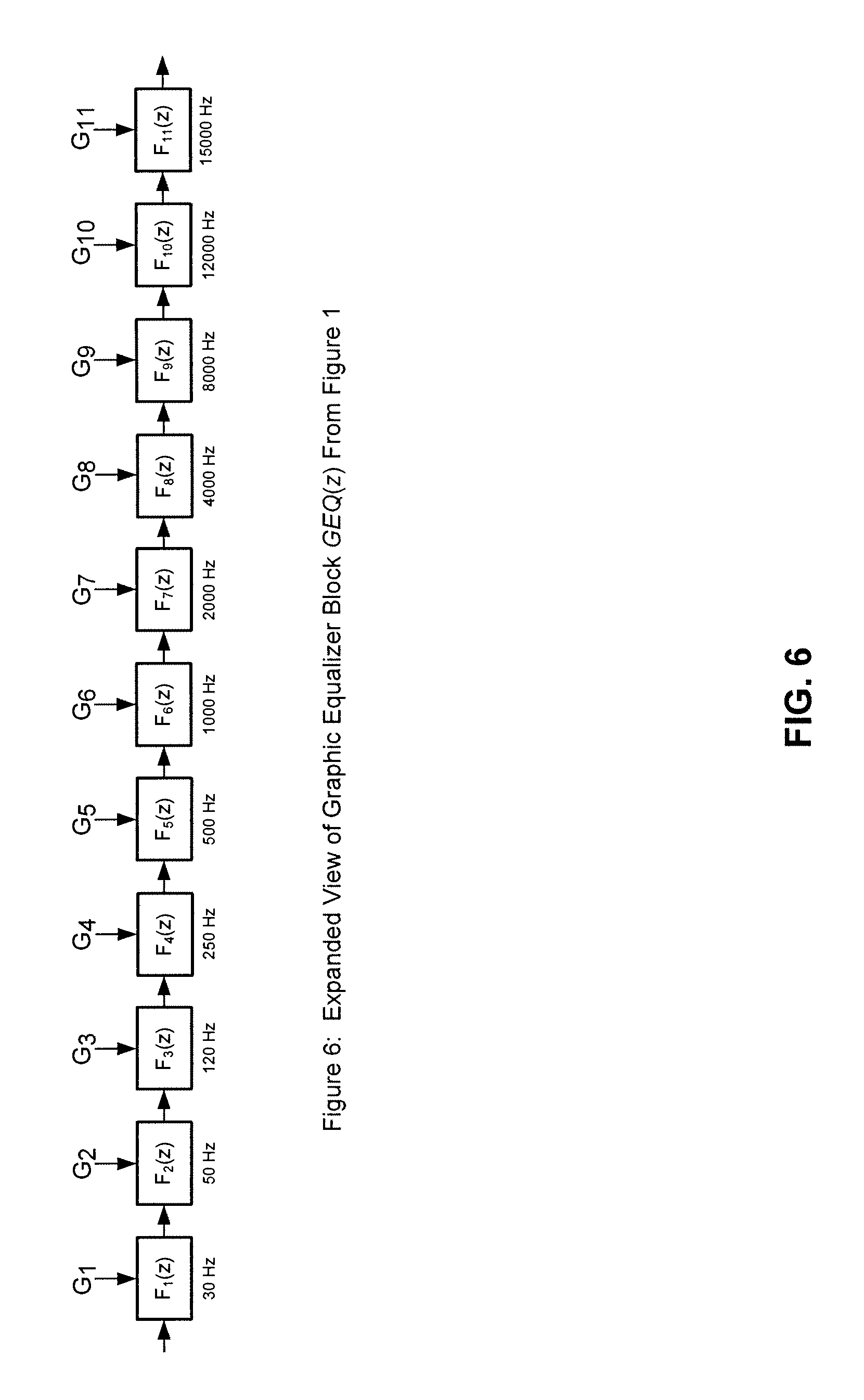
FIG. 5 illustrates the frequency response of a bell filter used in one embodiment of the digital signal processing method of the present invention.
FIG. 6 illustrates a block diagram of one embodiment of a graphic equalizer used in one embodiment of the digital signal processing method of the present invention.
FIG. 7 illustrates a block diagram showing how a filter can be constructed using the Mitra-Regalia realization.
FIG. 8 illustrates the effect of magnitude-complementary low-shelf filters that may be used in one embodiment of the digital signal processing method of the present invention.
FIG. 9 illustrates a block diagram of an implementation of a magnitude-complementary low-shelf filter that may be used in one embodiment of the digital signal processing method of the present invention.
FIG. 10 illustrates the static transfer characteristic (the relationship between output and input levels) of a compressor used in one embodiment of the digital signal processing method of the present invention.
FIG. 11 illustrates a block diagram of a direct form type 1 implementation of second order transfer function used in one embodiment of the digital signal processing method of the present invention.
FIG. 12 illustrates a block diagram of a direct form type 1 implementation of second order transfer function used in one embodiment of the digital signal processing method of the present invention.
FIG. 13 is a block diagram illustrating an example digital signal processing system in accordance with the systems and methods of the present invention.
The figures are not intended to be exhaustive or to limit the invention to the precise form disclosed. It should be understood that the invention can be practiced with modification and alteration, and that the invention be limited only by the claims and the equivalents thereof.
DETAILED DESCRIPTION OF THE PREFERRED EMBODIMENT
It is to be understood that the present invention is not limited to the particular methodology, compounds, materials, manufacturing techniques, uses, and applications described herein, as these may vary. It is also to be understood that the terminology used herein is used for the purpose of describing particular embodiments only, and is not intended to limit the scope of the present invention. It must be noted that as used herein and in the appended embodiments, the singular forms "a," "an," and "the" include the plural reference unless the context clearly dictates otherwise. Thus, for example, a reference to "an audio device" or separate device is a reference to one or more audio devices or separate devices that implement the systems and methods of the present invention, whether integrated or not and includes equivalents thereof known to those skilled in the art. Similarly, for another example, a reference to "a step" or "a means" is a reference to one or more steps or means and may include sub-steps and subservient means. All conjunctions used are to be understood in the most inclusive sense possible. Thus, the word "or" should be understood as having the definition of a logical "or" rather than that of a logical "exclusive or" unless the context clearly necessitates otherwise. Language that may be construed to express approximation should be so understood unless the context clearly dictates otherwise.
Unless defined otherwise, all technical and scientific terms used herein have the same meanings as commonly understood by one of ordinary skill in the art to which this invention belongs. Preferred methods, techniques, devices, and materials are described, although any methods, techniques, devices, or materials similar or equivalent to those described herein may be used in the practice or testing of the present invention. Structures described herein are to be understood also to refer to functional equivalents of such structures.
1.0 Overview
First, some background on linear time-invarient systems is helpful. A linear, time-invariant (LTI) discrete-time filter of order N with input x[k] and output y[k] is described by the following difference equation: y[k]=b.sub.0x[k]+b.sub.1x[k-1]+ . . . +b.sub.Nx[k-N]+a.sub.1y[k-1]+a.sub.2y[k-2]+ . . . +a.sub.Ny[k-N] where the coefficients {b0, b1, . . . , bN, a1, a2, . . . , aN} are chosen so that the filter has the desired characteristics (where the term desired can refer to time-domain behavior or frequency domain behavior).
The difference equation above can be excited by an impulse function, .delta.[k], whose value is given by
.delta..function..noteq. ##EQU00001##
When the signal .delta.[k] is applied to the system described by the above difference equation, the result is known as the impulse response, h[k]. It is a well-known result from system theory that the impulse response h[k] alone completely characterizes the behavior of a LTI discrete-time system for any input signal. That is, if h[k] is known, the output y[k] for an input signal x[k] can be obtained by an operation known as convolution. Formally, given h[k] and x[k], the response y[k] can be computed as
.function..infin..times..function..times..function. ##EQU00002##
Some background on the z-transform is also helpful. The relationship between the time-domain and the frequency-domain is given by a formula known as the z-transform. The z-transform of a system described by the impulse response h[k] can be defined as the function H(z) where
.function..infin..times..function..times. ##EQU00003##
and z is a complex variable with both real and imaginary parts. If the complex variable is restricted to the unit circle in the complex plane (i.e., the region described by the relationship [z|=1), what results is a complex variable that can be described in radial form as z=.di-elect cons..sup.j.theta., where 0.ltoreq..theta..ltoreq.2.pi. and j= {square root over (-1)}
Some background on the discrete-time Fourier transform is also instructive. With z described in radial form, the restriction of the z-transform to the unit circle is known as the discrete-time Fourier transform (DTFT) and is given by
.function. .times..times..theta..infin..times..function..times..times..times..theta. ##EQU00004##
Of particular interest is how the system behaves when it is excited by a sinusoid of a given frequency. One of the most significant results from the theory of LTI systems is that sinusoids are Eigen functions of such systems. This means that the steady-state response of an LTI system to a sinusoid sin(.theta.0k) is also a sinusoid of the same frequency .theta.0, differing from the input only in amplitude and phase. In fact, the steady-state output, yss[k] of the LTI system when driven by and input x[k]=sin(.theta.0k) is given by y.sub.ss[k]=A sin(.theta..sub.0k+.PHI..sub.0)
where A=|H(.di-elect cons..sup.j.theta..sub.0) and .PHI..sub.0=arg(H(e.sup.j.theta..sub.0)
Finally, some background on frequency response is needed. The equations above are significant because they indicate that the steady-state response of an LTI system when driven by a sinusoid is a sinusoid of the same frequency, scaled by the magnitude of the DTFT at that frequency and offset in time by the phase of the DTFT at that frequency. For the purposes of the present invention, what is of concern is the amplitude of the steady state response, and that the DTFT provides us with the relative magnitude of output-to-input when the LTI system is driven by a sinusoid. Because it is well-known that any input signal may be expressed as a linear combination of sinusoids (the Fourier decomposition theorem), the DTFT can give the response for arbitrary input signals. Qualitatively, the DTFT shows how the system responds to a range of input frequencies, with the plot of the magnitude of the DTFT giving a meaningful measure of how much signal of a given frequency will appear at the system's output. For this reason, the DTFT is commonly known as the system's frequency response.
2.0 Digital Signal Processing
FIG. 1 illustrates an example digital signal process flow of a method 100 according to one embodiment of the present invention. Referring now to FIG. 1, method 100 includes the following steps: input gain adjustment 101, first low shelf filter 102, first high shelf filter 103, first compressor 104, second low shelf filter 105, second high shelf filter 106, graphic equalizer 107, second compressor 108, and output gain adjustment 109.
In one embodiment, digital signal processing method 100 may take as input audio signal 110, perform steps 101-109, and provide output audio signal 111 as output. In one embodiment, digital signal processing method 100 is executable on a computer chip, such as, without limitation, a digital signal processor, or DSP. In one embodiment, such a chip may be one part of a larger audio device, such as, without limitation, a radio, MP3 player, game station, cell phone, television, computer, or public address system. In one such embodiment, digital signal processing method 100 may be performed on the audio signal before it is outputted from the audio device. In one such embodiment, digital signal processing method 100 may be performed on the audio signal after it has passed through the source selector, but before it passes through the volume control.
In one embodiment, steps 101-109 may be completed in numerical order, though they may be completed in any other order. In one embodiment, steps 101-109 may exclusively be performed, though in other embodiments, other steps may be performed as well. In one embodiment, each of steps 101-109 may be performed, though in other embodiments, one or more of the steps may be skipped.
In one embodiment, input gain adjustment 101 provides a desired amount of gain in order to bring input audio signal 110 to a level that will prevent digital overflow at subsequent internal points in digital signal processing method 100.
In one embodiment, each of the low-shelf filters 102, 105 is a filter that has a nominal gain of 0 dB for all frequencies above a certain frequency termed the corner frequency. For frequencies below the corner frequency, the low-shelving filter has a gain of .+-.G dB, depending on whether the low-shelving filter is in boost or cut mode, respectively. This is shown in FIG. 2.
In one embodiment, the systems and methods described herein may be implemented in a separate device that is located (e.g., wired or wirelessly) between, for example, a vehicle head unit, radio or other audio source and the vehicle's or other audio source's speaker system. This device may be installed at the factory. In another embodiment, however, this device may be retrofitted into a preexisting vehicle or other audio system. The device might also be used in conjunction with other audio or video equipment and speaker systems in addition to vehicle audio systems. For example, the device might be used in conjunction with a home stereo system and home stereo speakers or a vehicle DVD video/audio system and it may be wired or wireless.
FIG. 2 illustrates the effect of a low-shelf filter being implemented by one embodiment of the present invention. Referring now to FIG. 2, the purpose of a low-shelving filter is to leave all of the frequencies above the corner frequency unaltered, while boosting or cutting all frequencies below the corner frequency by a fixed amount, G dB. Also, note that the 0 dB point is slightly higher than the desired 1000 Hz. It is standard to specify a low-shelving filter in cut mode to have a response that is at -3 dB at the corner frequency, whereas a low-shelving filter in boost mode is specified such that the response at the corner frequency is at G-3 dB--namely, 3 dB down from maximum boost. Indeed, all of the textbook formulae for creating shelving filters lead to such responses. This leads to a certain amount of asymmetry, where for almost all values of boost or cut G, the cut and boost low-shelving filters are not the mirror images of one another. This is something that needed to be address by the present invention, and required an innovative approach to the filters' implementations.
Ignoring for now the asymmetry, the standard method for creating a low-shelving filter is as the weighted sum of high-pass and low-pass filters. For example, let's consider the case of a low-shelving filter in cut mode with a gain of -G dB and a corner frequency of 1000 Hz. FIG. 3 shows a high-pass filter with a 1000 cutoff frequency and a low-pass filter with a cutoff frequency of 1000 Hz, scaled by -G dB. The aggregate effect of these two filters applied in series looks like the low-shelving filter in FIG. 2. In practice, there are some limitations on the steepness of the transition from no boost or cut to G dB of boost or cut. FIG. 3 illustrates this limitation, with the corner frequency shown at 1000 Hz and the desired G dB of boost or cut not being achieved until a particular frequency below 1000 Hz. It should be noted that all of the shelving filters in the present invention are first-order shelving filters, which means they can usually be represented by a first-order rational transfer function:
.function..times..times. ##EQU00005##
In some embodiments, each of the high-shelf filters 103, 106 is nothing more than the mirror image of a low-shelving filter. That is, all frequencies below the corner frequency are left unmodified, whereas the frequencies above the corner frequency are boosted or cut by G dB. The same caveats regarding steepness and asymmetry apply to the high-shelving filter. FIG. 4 illustrates the effect of a high-shelf filter implemented by an embodiment of the present invention. Referring now to FIG. 4, a 1000 Hz high-shelving filter is shown.
FIG. 5 illustrates an example frequency response of a bell filter implemented by method 100 according to one embodiment of the present invention. As shown in FIG. 5, each of the second order filters achieves a bell-shaped boost or cut at a fixed center frequency, with F1(z) centered at 30 Hz, F11(z) centered at 16000 Hz, and the other filters in between centered at roughly one-octave intervals. Referring to FIG. 5, a bell-shaped filter is shown centered at 1000 Hz. The filter has a nominal gain of 0 dB for frequencies above and below the center frequency, 1000 Hz, a gain of -G dB at 1000 Hz, and a bell-shaped response in the region around 1000 Hz.
The shape of the filter is characterized by a single parameter: the quality factor, Q. The quality factor is defined as the ratio of the filter's center frequency to its 3-dB bandwidth, B, where the 3-dB bandwidth is illustrated as in the figure: the difference in Hz between the two frequencies at which the filter's response crosses the -3 dB point.
FIG. 6 illustrates an example graphic equalizer block 600 according to one embodiment of the present invention. Referring now to FIG. 6, graphic equalizer 600 consists of a cascaded bank of eleven second-order filters, F.sub.1(z), F.sub.2(z), . . . , F.sub.11(z). In one embodiment, graphic equalizer 107 (as shown in FIG. 1) is implemented as graphic equalizer 600.
One embodiment may have eleven second-order filters. In this embodiment each of eleven second-order filters might be computed from formulas that resemble this one:
.function..times..times..times..times. ##EQU00006##
Using such an equation results in one problem: each of the five coefficients above, {b.sub.0,b.sub.1,b.sub.2,a.sub.1,a.sub.2} depends directly on the quality factor, Q, and the gain, G. This means that for the filter to be tunable, that is, to have variable Q and G, all five coefficients must be recomputed in real-time. This can be problematic, as such calculations could easily consume the memory available to perform graphic equalizer 107 and create problems of excessive delay or fault, which is unacceptable. This problem can be avoided by utilizing the Mitra-Regalia Realization.
A very important result from the theory of digital signal processing (DSP) is used to implement the filters used in digital signal processing method 100. This result states that a wide variety of filters (particularly the ones used in digital signal processing method 100) can be decomposed as the weighted sum of an allpass filter and a feed forward branch from the input. The importance of this result will become clear. For the time being, suppose that a second-order transfer function, H(z), is being implemented to describes a bell filter centered at fc with quality factor Q and sampling frequency Fs by
.function..times..times..times..times. ##EQU00007##
Ancillary quantities k1, k2 can be defined by
.function..pi..times..times..function..pi..times..times. ##EQU00008## .function..times..pi..times..times. ##EQU00008.2##
and transfer function, A(z) can be defined by
.function..function..times..function..times..times..times. ##EQU00009##
A(z) can be verified to be an allpass filter. This means that the amplitude of A(z) is constant for all frequencies, with only the phase changing as a function of frequency. A(z) can be used as a building block for each bell-shaped filter. The following very important result can be shown: H(z)=1/2(1+G)A(z)+1/2(1-G)
This is the crux of the Mitra-Regalia realization. A bell filter with tunable gain can be implemented to show the inclusion of the gain G in a very explicit way. This is illustrated in FIG. 7, which illustrates an example filter constructed using the Mitra-Regalia realization according to one embodiment of the present invention.
There is a very good reason for decomposing the filter in such a non-intuitive manner. Referring to the above equation, every one of the a and b coefficients needs to be re-computed whenever G gets changed (i.e., whenever one of the graphic EQ "slider" is moved). Although the calculations that need to be performed for the a and b coefficients have not been shown, they are very complex and time-consuming and it simply is not practical to recompute them in real time. However, in a typical graphic EQ, the gain G and quality factor Q remain constant and only G is allowed to vary. A(z) does not depend in any way on the gain, G and that if Q and the center-frequency fc remain fixed (as they do in a graphic EQ filter), then k1 and k2 remain fixed regardless of G. Thus, these variables only need to be computed once. Computing the gain variable is accomplished by varying a couple of simple quantities in real time: 1/2(1+G) and 1/2(1-G)
These are very simple computations and only require a couple of CPU cycles. This leaves only the question of how to implement the allpass transfer function, A(z). The entire graphic equalizer bank thus consists of 11 cascaded bell filters, each of which is implemented via its own Mitra-Regalia realization:
.function.>.times..times..times..times..function.>.times..times..ti- mes..times..function.>.times..times..times..times. ##EQU00010##
It can be seen from that equation that the entire graphic equalizer bank depends on a total of 22 fixed coefficients that need to be calculated only once and stored in memory. The "tuning" of the graphic equalizer is accomplished by adjusting the parameters G1, G2, . . . , G11. See FIG. 6 to see this in schematic form. The Mitra-Regalia realization may be used over and over in the implementation of the various filters used digital signal processing method 100. Mitra-Regalia may also be useful in implementing the shelving filters, where it is even simpler because the shelving filters use first-order filter. The net result is that a shelving filter is characterized by a single allpass parameter, k, and a gain, G. As with the bell filters, the shelving filters are at fixed corner frequencies (in fact, all of them have 1 kHz as their corner frequency) and the bandwidth is also fixed. All told, four shelving filters are completely described simply by H.sub.1(z).fwdarw.fixed k.sup.1, variable G.sub.1 H.sub.2(z).fwdarw.fixed k.sup.2, variable G.sub.2 H.sub.3(z).fwdarw.fixed k.sup.3, variable G.sub.3 H.sub.4(z).fwdarw.fixed k.sup.4,variable G.sub.4
As discussed above, there is an asymmetry in the response of a conventional shelving filter when the filter is boosting versus when it is cutting. This is due, as discussed, to the design technique having different definitions for the 3-dB point when boosting than when cutting. Digital signal processing method 100 relies on the filters H1(z) and H3(z) being the mirror images of one another and the same holds for H2(z) and H4(z). This led to the use of a special filter structure for the boosting shelving filters, one that leads to perfect magnitude cancellation for H1, H3 and H2, H4, as shown in FIG. 8. This type of frequency response is known as magnitude complementary. This structure is unique to the present invention. In general, it is a simple mathematical exercise to derive for any filter H(z) a filter with complementary magnitude response. The filter H-1(z) works, but may not be stable or implementable function of z, in which case the solution is merely a mathematical curiosity and is useless in practice. This is the case with a conventional shelving filter. The equations above show how to make a bell filter from an allpass filter. These equation applies equally well to constructing a shelving filter beginning with a first-order allpass filter, A(z), where
.function..alpha..alpha..times..times. ##EQU00011## and .alpha. is chosen such that
.alpha..function..times..pi..times..times..function..times..pi..times..ti- mes. ##EQU00012##
where fc is the desired corner frequency and Fs is the sampling frequency. Applying the above equations and re-arranging terms, this can be expressed as
.function..times..times..function. ##EQU00013##
This is the equation for a low-shelving filter. (A high-shelving filter can be obtained by changing the term (1-G) to (G-1)). Taking the inverse of H(z) results in the following:
.function..times..times..function. ##EQU00014##
This equation is problematic because it contains a delay-free loop, which means that it cannot be implemented via conventional state-variable methods. Fortunately, there are some recent results from system theory that show how to implement rational functions with delay-free loops. Fontana and Karjalainen (IEEE Signal Processing Letters, Vol. 10, No. 4, April 2003) show that each step can be "split" in time into two "sub-steps."
FIG. 9 illustrates an example magnitude-complementary low-shelf filter according to one embodiment of the present invention. During the first sub-step (labeled "subsample 1"), feed filter A(z) with zero input and compute its output, 10[k]. During this same subsample, calculate the output y[k] using the value of 10[k], which from the equation immediately above can be performed as follows:
.function..times..alpha..times..times..times..times..function..times..fun- ction..times..alpha..function..times..function..times..function. ##EQU00015##
It can be seen from FIG. 9 that these two calculations correspond to the case where the switches are in the "subsample 1" position. Next, the switches are thrown to the "subsample 2" position and the only thing left to do is update the internal state of the filter A(z). This unconventional filter structure results in perfect magnitude complementarity, 11. This can be exploited for the present invention in the following manner: when the shelving filters of digital signal processing method 100 are in "cut" mode, the following equation can be used:
.function..times..times..function. ##EQU00016##
However, when the shelving filters of digital signal processing method 100 are in "boost" mode, the following equation can be used with the same value of G as used in "cut" mode:
.function..times..alpha..times..times..times..function..times..function..- times..alpha..function..times..function..times..function. ##EQU00017##
This results in shelving filters that are perfect mirror images of one another, as illustrated in FIG. 8, which is what is needed for digital signal processing method 100. (Note: Equation 16 can be changed to make a high-shelving filter by changing the sign on the (1-G)/2 term). FIG. 8 illustrates the effect of a magnitude-complementary low-shelf filter implemented by an embodiment of the present invention.
Each of the compressors 104, 108 is a dynamic range compressor designed to alter the dynamic range of a signal by reducing the ratio between the signal's peak level and its average level. A compressor is characterized by four quantities: the attack time, Tatt, the release time, Trel, the threshold, KT, and the ratio, r. In brief, the envelope of the signal is tracked by an algorithm that gives a rough "outline" of the signal's level. Once that level surpasses the threshold, KT, for a period of time equal to Tatt, the compressor decreases the level of the signal by the ratio r dB for every dB above KT. Once the envelope of the signal falls below KT for a period equal to the release time, Trel, the compressor stops decreasing the level. FIG. 10 illustrates a static transfer characteristic (relationship between output and input levels) of a compressor implemented in accordance with one embodiment of the present invention.
It is instructive to examine closely the static transfer characteristic. Assume that the signal's level, L[k] at instant k has been somehow computed. For instructive purposes, a one single static level, L, will be considered. If L is below the compressor's trigger threshold, KT, the compressor does nothing and allows the signal through unchanged. If, however, L is greater than KT, the compressor attenuates the input signal by r dB for every dB by which the level L exceeds KT.
It is instructive to consider an instance where L is greater than KT, which means that 20 log.sub.10(L)>20 log.sub.10(KT). In such an instance, the excess gain, i.e., the amount in dB by which the level exceeds the threshold, is: g.sub.excess=20 log.sub.10(L)-20 log.sub.10(KT). As the compressor attenuates the input by r dB for every dB of excess gain, the gain reduction, gR, can be expressed as
.times..times..function..times..times..function. ##EQU00018##
From that, it follows that that with the output of the compressor, y given by 20 log.sub.10(y)=gR*20 log.sub.10(x), that the desired output-to-input relationship is satisfied.
Conversion of this equation to the linear, as opposed to the logarithmic, domain yields the following:
.function..times..times..function..function. ##EQU00019##
The most important part of the compressor algorithm is determining a meaningful estimate of the signal's level. This is accomplished in a fairly straightforward way: a running "integration" of the signal's absolute value is kept, where the rate at which the level is integrated is determined by the desired attack time. When the instantaneous level of the signal drops below the present integrated level, the integrated level is allowed to drop at a rate determined by the release time. Given attack and release times Tatt and Trel, the equation used to keep track of the level, L[k] is given by
.function..alpha..function..alpha..times..function..times..times..times..- times..function..gtoreq..function..alpha..function..alpha..times..function- ..times..times..times..times..function.<.function..times..times..times.- .times..alpha..function..times..times..times..times..times..alpha..functio- n..times..times..times. ##EQU00020##
At every point of the level calculation as described above, L[k] as computed is compared to the threshold KT, and if L[k] is greater than KT, the input signal, x[k], is scaled by an amount that is proportional to the amount by which the level exceeds the threshold. The constant of proportionality is equal to the compressor ratio, r. After a great deal of mathematical manipulation, the following relationship between the input and the output of the compressor is established:
With the level L[k] as computed using, for example, the equation for L[k], above, the quantity Gexcess by is computed as G.sub.excess=L[k]K.sub.T.sup.-1
which represents the amount of excess gain. If the excess gain is less than one, the input signal is not changed and passed through to the output. In the event that the excess gain exceeds one, the gain reduction, GR is computed by:
.times..function..times. ##EQU00021##
and then the input signal is scaled by GR and sent to the output: output[k]=G.sub.Rx[k]
Through this procedure, an output signal whose level increases by 1/r dB for every 1 dB increase in the input signal's level is created.
In practice, computing the inverse K.sub.T.sup.-1 for the above equations can be time consuming, as certain computer chips are very bad at division in real-time. As KT is known in advance and it only changes when the user changes it, a pre-computed table of K.sub.T.sup.-1 values can be stored in memory and used as needed. Similarly, the exponentiation operation in the above equation calculating GR is extremely difficult to perform in real time, so pre-computed values can be used as an approximation. Since quantity GR is only of concern when Gexcess is greater than unity, a list of, say, 100 values of GR, pre-computed at integer values of GR from GR=1 to GR=100 can be created for every possible value of ratio r. For non-integer values of GR (almost all of them), the quantity in the above equation calculating GR can be approximated in the following way. Let interp be the amount by which Gexcess exceeds the nearest integral value of Gexcess. In other words, interp=G.sub.excess-[(G.sub.excess)]
and let GR,0 and GR,1 refer to the pre-computed values
##EQU00022## ##EQU00022.2## ##EQU00022.3##
Linear interpolation may then be used to compute an approximation of GR as follows: G.sub.R=G.sub.R,0 interp*(G.sub.R,1-G.sub.R,0)
The error between the true value of GR and the approximation in the above equation can be shown to be insignificant for the purposes of the present invention. Furthermore, the computation of the approximate value of GR requires only a few arithmetic cycles and several reads from pre-computed tables. In one embodiment, tables for six different values of ratio, r, and for 100 integral points of Gexcess may be stored in memory. In such an embodiment, the entire memory usage is only 600 words of memory, which can be much more palatable than the many hundred cycles of computation that would be necessary to calculate the true value of GR directly. This is a major advantage of the present invention.
Each of the digital filters in digital signal processing method 100 may be implemented using any one of a variety of potential architectures or realizations, each of which has its trade-offs in terms of complexity, speed of throughput, coefficient sensitivity, stability, fixed-point behavior, and other numerical considerations. In a specific embodiment, a simple architecture known as a direct-form architecture of type 1 (DF1) may be used. The DF1 architecture has a number of desirable properties, not the least of which is its clear correspondence to the difference equation and the transfer function of the filter in question. All of the digital filters in digital signal processing method 100 are of either first or second order.
The second-order filter will be examined in detail first. As discussed above, the transfer function implemented in the second-order filter is given by
.function..times..times..times..times. ##EQU00023##
which corresponds to the difference equation y[k]=b.sub.0x[k]+b.sub.1x[k-1]+b.sub.2x[k-2]-a.sub.1y[k-1]-a.sub.2y[k-2]
FIG. 11 illustrates the DF1 architecture for a second-order filter according to one embodiment of the present invention. As shown in FIG. 11, the multiplier coefficients in this filter structure correspond to the coefficients in the transfer function and in the difference equation above. The blocks marked with the symbol z-1 are delay registers, the outputs of which are required at every step of the computation. The outputs of these registers are termed state variables and memory is allocated for them in some embodiments of digital signal processing method 100. The output of the digital filter is computed as follows:
Initially, each of the state variables is set to zero. In other words, x[-1]=x[-2]=y[-1]=y[-2]=0.
At time k=0 the following computation is done, according to FIG. 11: y[0]=b.sub.0x[0]+b.sub.1x[-1]+b.sub.2x[-2]-a.sub.1y[-1]-a.sub.2y[-2].
Then, the registers are updated so that the register marked by x[k-1] now holds x[0], the register marked by x[k-2] now holds x[-1], the register marked by y[k-1] holds y[0], and the register marked by y[k-2] holds y[-1].
At time k=1 the following computation is done: y[1]=b.sub.0x[1]+b.sub.1x[0]+b.sub.2x[-1]-a.sub.1y[0]-a.sub.2y[-1].
Then, the register update is again completed so that the register marked by x[k-1] now holds x[1], the register marked by x[k-2] now holds x[0], the register marked by y[k-1] holds y[1], and the register marked by y[k-2] holds y[0].
This process is then repeated over and over for all instants k: A new input, x[k], is brought in, a new output y[k] is computed, and the state variables are updated.
In general, then, the digital filtering operation can be viewed as a set of multiplications and additions performed on a data stream x[0], x[1], x[2], . . . using the coefficients b0, b1, b2, a1, a2 and the state variables x[k-1], x[k-2], y[k-1], y[k-2].
The manifestation of this in specific situations is instructive. Examination of the bell filter that constitutes the fundamental building-block of graphic equalizer 107 is helpful. As discussed above, the bell filter is implemented with a sampling frequency Fs, gain G at a center frequency fc, and quality factor Q as H(z)=1/2(1+G)A(z)+1/2(1-G)
where A(z) is an allpass filter defined by
.function..function..times..function..times..times. ##EQU00024##
where k1 and k2 are computed from fc and Q via the equations
.function..pi..times..times..function..pi..times..times. ##EQU00025## ##EQU00025.2## .function..times..pi..times..times. ##EQU00025.3##
The values k1 and k2 are pre-computed and stored in a table in memory. To implement a filter for specific values of Q and fc, the corresponding values of k1 and k2 are looked up in this table. Since there are eleven specific values of fc and sixteen specific values of Q in the algorithm, and the filter operates at a single sampling frequency, Fs, and only k2 depends on both fc and Q, the overall storage requirements for the k1 and k2 coefficient set is quite small (11.times.16.times.2 words at worst).
Observe from the equation above for A(z) that its coefficients are symmetric. That is, the equations can be re-written as
.function..times..times..times..times..times..times..times..times..times.- .times..times..times..times..times. ##EQU00026## ##EQU00026.2## .times..times. ##EQU00026.3## ##EQU00026.4## .times..times..function. ##EQU00026.5##
Observe that A(z) as given in the above equation implies the difference equation y[k]=geq.sub.b0(x[k]+geq.sub.b1x[k-1]+x[k-2]-geq.sub.b1y[k-1]-ge- q.sub.b0y[k-2]
which can be rearranged to yield y[k]=geq.sub.b0(x[k]-y[k-2])+geq.sub.b1(x[k-1]-y[k-1])+x[k-2]
In a specific embodiment, the state variables may be stored in arrays xv[ ] and yv[ ] with xv[0] corresponding to x[k-2], xv[1] corresponding to x[k-1], yv[0] corresponding to y[k-2] and yv[1] corresponding to y[k-1]. Then the following code-snippet implements a single step of the allpass filter:
TABLE-US-00001 void allpass(float *xv, float *yv, float *input, float *output) { *output = geq_b0 * (*input - yv[0]) + geq_b1 * (xv[1] - yv[1]) + xv[0] xv[0] = xv[1]; \\ update xv[1] = *input; \\ update yv[0] = yv[1]; \\update yv[1] = *output; \\update }
Now the loop may be incorporated around the allpass filter as per the equations above. This is trivially realized by the following:
TABLE-US-00002 void bell(float *xv, float *yv, float gain, float *input, float *output) { allpass(xv, yv, input, output); *output = 0.5 * (1.0-gain) * (*output) + 0.5 * (1.0+gain) * (*input); }
More concisely, the previous two code snippets can be combined into a single routine that looks like this:
TABLE-US-00003 void bell(float *xv, float *yv, float gain, float *input, float *output) { float ap_output = geq_b0 * (*input - yv[0]) + geq_b1 * (xv[1] - yv[1]) + xv[0] xv[0] = xv[1]; \\ update xv[1] = *input; \\ update yv[0] = yv[1]; \\update yv[1] = *output; \\update *output = 0.5 * (1.0-gain) * ap_output + 0.5 * (1.0+gain) * (*input); }
The first-order filter will now be examined in detail. These filters can be described by the transfer function
.function..times..times. ##EQU00027##
which corresponds to the difference equation y[k]=b.sub.0x[k]+b.sub.1x[k-1]-a.sub.1y[k-1].
FIG. 12 illustrates the DF1 architecture for a first-order filter according to one embodiment of the present invention. Referring now to FIG. 12, the multiplier coefficients in this filter structure correspond in a clear way to the coefficients in the transfer function and in the difference equation. The output of the digital filter is computed as follows:
Initially, every one of the state variables is set to zero. In other words, x[-1]=y[-1]=0.
At time k=0 the following computation is done, according to FIG. 11: y[0]=b.sub.0x[0]+b.sub.1x[-1]-a.sub.1y[-1].
Then, the registers are updated so that the register marked by x[k-1] now holds x[0], and the register marked by y[k-1] holds y[0].
At time k=1 the following computation is done: y[1]=b.sub.0x[1]+b.sub.1x[0]-a.sub.1y[0].
Then, the register update is again completed so that the register marked by x[k-1] now holds x[1] and the register marked by y[k-1] holds y[1].
This process is then repeated over and over for all instants k: A new input, x[k], is brought in, a new output y[k] is computed, and the state variables are updated.
In general, then, the digital filtering operation can be viewed as a set of multiplications and additions performed on a data stream x[0], x[1], x[2], . . . using the coefficients b0, b1, a1 and the state variables x[k-1], y[k-1].
FIG. 13 is a block diagram illustrating an example digital signal processing system 1300 in accordance with the systems and methods described herein. Referring now to FIG. 13, the example digital signal processing system 1300 may process wireless input signals 1302 that are input into a wireless receiver 1304. The wireless signals 1302 may be amplitude modulation signals, frequency modulation signals, digitally modulated signals, or other types of transmitted signals. The wireless receiver 1304 may be configured to receive the type of wireless input signal used, e.g., digitally modulated signals, etc.
In various embodiments, the wireless receiver 1304 may receive the wireless input signal 1302 and conditions it prior to processing by a digital processing device such as the digital signal processor (DSP) 1306. For example, in some embodiments, high-level amplified signals may be conditioned to reduce the signal's range so that they are not outside the dynamic range of the analog-to-digital converters. The conditioned signal may then be input into a DSP 1306.
The DSP block 1306 may include necessary components for processing the input signals as described herein. For example, the DSP 1306 may run various digital processing algorithms, including, for example, noise cancellation algorithms other algorithms described herein. These algorithms may process audio signals to produce studio-quality sound.
The DSP 1306 may be coupled to an amplifier 1308 that amplifies the processed audio signal and provides an output signal for the headphone drivers 1310. In some embodiments, the amplifier 1308 may include a multi-channel amplification section, such as a stereo amplifier. In some examples, multiple stereo amplifiers may be used.
In the amplifier 1308, the level of the output signal may be raised so that it may be reproduced using the headphone driver 1310 to drive audio transducers, e.g., a pair of headphones. The audio transducer may be used to provide sound to a listener.
Headphones may include earphones, earbuds, stereophones, and headsets. The headphones generally comprise a pair of small loudspeakers, or, in some embodiments, a single speaker. The small loudspeaker or loudspeakers may be formed such that a user can hold them close to or within a user's ears. The headphones can include a connection device, such as a connector to connect the headphones to, e.g., an audio signal source such as the headphone driver 1310. In some cases, the headphones used may be wireless headphones. In such an embodiment, a separate transmitter (not shown) can be connected to headphone drivers 1310. This transmitter can then transmit a signal to the wireless headphone. This can allow a person wearing the headphones to move about more freely without having to be concerned for wires, which may get in the way or limit movement. Additionally, some embodiments may include noise cancellation headphones.
In other embodiments, a connector, e.g., a headphone connector might be used in conjunction with other circuitry to drive other types of audio transducers, such as speakers including full range drivers, subwoofers, woofers, mid-range drivers, and tweeters. These speakers might be horn loudspeakers, piezoelectric speakers, electrostatic loudspeakers, ribbon and planar magnetic loudspeakers, bending wave loudspeakers, flat panel loudspeakers, distributed mode loudspeakers, Keil air motion transducers, or plasma arc speakers, to name a few. The speakers may be included in speaker enclosures, headphones, etc.
In certain embodiments, a power supply 1312 may provide power to the circuit DSP 1306, amplifier, as well as other circuit elements, such as the system clocks 1314, mater control unit 1316, and the wireless receiver 1304. In some embodiments, the power supply includes a battery that may store and provide power. The power from this battery, or other power source, such as a home alternating current power source, can be conditioned in the power supply 1312. In embodiments that use a battery to provide power, the power supply 1312 may also include various circuitry to charge the battery.
The systems clocks 1314 generate and provide timing signals, e.g., clock signals to control the timing in the device 1300. A crystal or other oscillator may be used to generate the system clocks 1304. In some examples, a master clock may be divided to generate the needed clock signals.
The systems and methods described herein may include a power supply circuit 1312. The power supply circuitry 1312 takes supplied voltage, converts and conditions it and provides power for various circuits used to process the audio signals.
A master control unit (MCU) 1316 can be used to control the overall functionality of the device 1300. For example, in some embodiments, the MCU 1316 may boot, run, and control other circuits in the device 1300.
In some embodiments, the systems and methods described herein may be used in a device external to a personal listening device, such as a set of headphones. In this way, the external device may drive the headphones and allow a listener to listen to, e.g., music. In other embodiments, the systems and methods described herein may be incorporated into a set of headphones. These systems and methods may be incorporated into, e.g., a set of headphones via a DSP in the headphone circuitry. This may allow a manufacturer or user in the context where the systems and methods are used in vehicles (e.g., Ford, GM, Toyota, Hyundai, etc.) the ability to create a custom profile or `sound` for their specific vehicles and/or brands or types of vehicles (cars, trucks, SUVs, buses, RV's, military vehicles, such as tanks) and/or product lines. For example, in some cases a user might own multiple vehicles and might want each vehicle to provide a similar sound experience when using headphones in each of the vehicles. Alternatively, a user might want the sound experience while using the headphones to be the same or similar to a sound experience in a particular car when headphones are not used, e.g., when a head unit and speakers are used with the systems and methods described herein to produce, for example, studio quality sound. Accordingly, in some embodiments, the systems and methods described herein might be used to create the same or similar sound experience across multiple vehicles, using either headphones or speakers.
In some examples, the manufacturer or user can create profiles to suit the tastes of their customer and the vehicles they use or purchase. In other embodiments, the users of the headphones or other personal listening device may create their own profile by, for example, using a pair of headphones incorporating these systems and methods to listen to music and adjusting the system based on, for example, personal preferences. For example, when a user listens to music using the headphones or other personal listening device, they might adjust the processing of the music by adjusting a first low shelf filter, a first compressor, or a graphic equalizer. They might also change the processing of the music signal by adjusting a second compressor and adjust the gain of the compressed signal after the second compressor. In some examples, the user may adjust an amplifier that increases the amplitude of the signal into an input of headphone drivers.
Various embodiments of these systems and methods may be used in conjunction with vehicles in addition to cars, such as pickup trucks, SUV's, trucks, tractors, buses, etc. In some examples, these systems and methods may also be used in conjunction with aviation and marine applications. In various embodiments, these systems and methods may also be used in other areas were, e.g., headphones might be used to listen to music, for example, homes, offices, trailers, etc.
Referring back to the equations above, a first-order shelving filter can be created by applying the equation
.function..function..times..function..times..times. ##EQU00028##
to the first-order allpass filter A(z), where
.function..alpha..alpha..times..times. ##EQU00029##
where .alpha. is chosen such that
.alpha..function..times..pi..times..times..function..times..pi..times..ti- mes. ##EQU00030##
where fc is the desired corner frequency and Fs is the sampling frequency. The allpass filter A(z) above corresponds to the difference equation y[k]=.alpha.x[k]-x[k-1]+.alpha.y[k-1].
If allpass coefficient .alpha. is referred to as allpass coef and the equation terms are rearranged, the above equation becomes y[k]=allpass_coef(x[k]+y[k-1]-x[k-1].
This difference equation corresponds to a code implementation of a shelving filter that is detailed below.
One specific software implementation of digital signal processing method 100 will now be detailed.
Input gain adjustment 101 and output gain adjustment 109, described above, may both be accomplished by utilizing a "scale" function, implemented as follows:
TABLE-US-00004 void scale(gain, float *input, float *output) { for (i = 0; i < NSAMPLES; i++) { *output++ = inputGain * (*input++);} }
First low shelf filter 102 and second low shelf filter 105, described above, may both be accomplished by utilizing a "low shelf" function, implemented as follows:
TABLE-US-00005 void low_shelf(float *xv, float *yv, float *wpt, float *input, float *output) { float l; int i; for (1 = 0; i < NSAMPLES; i++) { if (wpt[2] < 0.0) \\ cut mode, use conventional realization { \\ allpass_coef = alpha yv[0] = ap_coef * (*input) + (ap_coef * ap_coef - 1.0) * xv[0]; xv[0] = ap_coef * xv[0] + *input; *output++ = 0.5 * ((1.0 + wpt[0]) * (*input++) + (1.0 - wpt[0]) * yv[0]); } else \\ boost mode, use special realization { 1 = (ap_coef * ap_coef - 1.0) * xv[0]; *output = wpt[1] * ((*input++) - 0.5 * (1.0 - wpt[0]) * 1); xv[0] = ap_coef * xv[0] + *output++; } } }
As this function is somewhat complicated, a detailed explanation of it is proper. First, the function declaration provides:
void low_shelf(float*xv, float*yv, float*wpt,
float*input,float*output)
The "low_shelf" function takes as parameters pointers to five different floating-point arrays. The arrays xv and yv contain the "x" and "y" state variables for the filter. Because the shelving filters are all first-order filters, the state-variable arrays are only of length one. There are distinct "x" and "y" state variables for each shelving filter used in digital signal processing method 100. The next array used is the array of filter coefficients "wpt" that pertain to the particular shelving filter. wpt is of length three, where the elements wpt[0], wpt[1], and wpt[2] describe the following: wpt[0]=G wpt[1]=2[(1+G)+.alpha.(1-G)].sup.-1 wpt[2]=-1 when cutting, 1 when boosting
and .alpha. is the allpass coefficient and G is the shelving filter gain. The value of .alpha. is the same for all shelving filters because it is determined solely by the corner frequency (it should be noted that and all four of the shelving filters in digital signal processing method 100 have a corner frequency of 1 kHz). The value of G is different for each of the four shelving filters.
The array "input" is a block of input samples that are fed as input to each shelving filter, and the results of the filtering operation are stored in the "output" array.
The next two lines of code,
Float 1;
int i;
allocate space for a loop counter variable, i, and an auxiliary quantity, 1, which is the quantity 10[k] from FIG. 9.
The next line of code,
for (i=0; i<NSAMPLES; i++)
performs the code that follows a total of NSAMPLES times, where NSAMPLES is the length of the block of data used in digital signal processing method 100.
This is followed by the conditional test
if (wpt[2]<0,0)
and, recalling the equations discussed above, wpt[2]<0 corresponds to a shelving filter that is in "cut" mode, whereas wpt[2]>=0 corresponds to a shelving filter that is in "boost" mode. If the shelving filter is in cut mode the following code is performed:
TABLE-US-00006 if (wpt[2] < 0.0) \\ cut mode, use conventional realization { \\ allpass_coef = alpha yv[0] = ap_coef * (*input) + (ap_coef * ap_coef - 1.0) * xv[0]; xv[0] = ap_coef * xv[0] + *input; *output++ = 0.5 * ((1.0 + wpt[0]) * (*input++) + (1.0 - wpt[0]) * yv[0]); }
The value xv[0] is simply the state variable x[k] and yv[0] is just yv[k]. The code above is merely an implementation of the equations y[k]=.alpha.in[k]+(a.sup.2-1)x[k] x[k]=.alpha.x[k]+in[k] out[k]=1/2((1+G)in[k]+(1-G)y[k])
If the shelving filter is in cut mode the following code is performed:
TABLE-US-00007 else \\ boost mode, use special realization { 1 = (ap_coef * ap_coef - 1.0) * xv[0]; *output = wpt[1] * ((*input++) - 0.5 * (1.0 - wpt[0]) * 1); xv[0] = ap_coef * xv[0] + *output++; }
which implements the equations i.sub.0[k]=(.alpha..sup.2-1)x[k] out[k]=2[(1+G)+.alpha.(1-G)].sup.-1in[k]-1/2(1-G)i.sub.0[k] x[k]=.alpha.x[k-1]+out[k]
First high shelf filter 103 and second high shelf filter 106, described above, may both be accomplished by utilizing a "high_shelf" function, implemented as follows:
TABLE-US-00008 void high_shelf(float *xv, float *yv, float *wpt, float *input, float *output) { float l; int i; for (i = 0; i < NSAMPLES; i++) { if (wpt[2] < 0.0) \\ cut mode, use conventional realization, { \\ allpass_coef = alpha yv[0] = allpass_coef * (*input) + (allpass_coef * allpass_coef - 1.0) * xv[0]; xv[0] = allpass_coef * xv[0] + *input; *output++ = 0.5 * ((1.0 + wpt[0]) * (*input++) - (1.0 - wpt[0]) * yv[0]); } else \\ boost mode, use special realization { l = (allpass_coef * allpass_coef - 1.0) * xv[0]; *output = wpt[1] * ((*input++) + 0.5 * (1.0 - wpt[0]) * l); xv[0] = allpass_coef * xv[0] + *output++; } } }
Implementing the high-shelving filter is similar to implementing the low-shelving filter. Comparing the two functions above, the only substantive difference is in the sign of a single coefficient. Therefore, the program flow is identical.
Graphic equalizer 107, described above, may be implemented using a series of eleven calls to a "bell" filter function, implemented as follows:
TABLE-US-00009 void bell(float *xv, float *yv, float *wpt, float *input, float *output) { float geq_gain = wpt[0]; \\ G float geq_b0 = wpt[1]; \\ k2 float geq_b1 = wpt[2]; \\ k1(1+k2) float ap_output; int i; for (1 = 0; i < NSAMPLES; i++) { ap_output = geq_b0 * (*input - yv[0]) + geq_b1 * (xv[1] - yv[1]) + xv[0]; xv[0] = xv[1]; \\ update xv[1] = *input; \\ update yv[0] = yv[1]; \\update yv[1] = *output; \\update *output++ = 0.5 * (1.0-gain) * ap_output + 0.5 * (1.0+gain) * (*input++); } }
The function bell( ) takes as arguments pointers to arrays xv (the "x" state variables), yv (the "y" state variables), wpt (which contains the three graphic EQ parameters G, k2, and k1(1+k2)), a block of input samples "input", and a place to store the output samples. The first four statements in the above code snippet are simple assignment statements and need no explanation.
The for loop is executed NSAMPLES times, where NSAMPLES is the size of the block of input data. The next statement does the following: ap.sub.output=geq.sub.b0*(*input-yv[0])+geq.sub.b1*(xv[1]-yv[1])+xv[0]
The above statement computes the output of the allpass filter as described above. The next four statements do the following:
xv[0]=xv[1];
shifts the value stored in x[k-1] to x[k-2].
xv[1]=*input;
shifts the value of input[k] to x[k-1].
yv[0]=yv[1];
shifts the value stored in y[k-1] to y[k-2].
yv[1]=*output;
shifts the value of output[k], the output of the allpass filter, to y[k-1].
Finally, the output of the bell filter is computed as *output++=0.5*(1.0-gain)*ap_output+0.5*(1.0+gain)*(*input++);
First compressor 104 and second compressor 108, described above, may be implemented using a "compressor" function, implemented as follows:
TABLE-US-00010 void compressor(float *input, float *output, float *wpt, int index) { static float level; float interp, GR, excessGain, L, invT, ftempabs; invT = wpt[2]; int i, j; for (i = 0; i < NSAMPLES; i ++) { ftempabs = fabs(*input++); level = (ftempabs >= level)? wpt[0] * (level - ftempabs) + ftempabs : wpt[1] * (level - ftempabs) + ftempabs; GR = 1.0; if (level * invT > 1.0) { excessGain = level *invT; interp = excessGain - trunc(excessGain); j = (int) trunc(excessGain) - 1; if (j < 99) { GR = table[index][j] + interp * (table[index][j+1] - table[index][j]); // table[ ][ ] is the exponentiation table } else { GR = table[index][99]; } } *output++ = *input++ * GR; } }
The compressor function takes as input arguments pointers to input, output, and wpt arrays and an integer, index. The input and output arrays are used for the blocks of input and output data, respectively. The first line of code,
static float level;
allocates static storage for a value called "level" which maintains the computed signal level between calls to the function. This is because the level is something that needs to be tracked continuously, for the entire duration of the program, not just during execution of a single block of data.
The next line of code,
float interp, GR, excessGain, L, invT, ftempabs;
allocates temporary storage for a few quantities that are used during the computation of the compressor algorithm; these quantities are only needed on a per-block basis and can be discarded after each pass through the function.
The next line of code,
invT=wpt[2];
extracts the inverse of the compressor threshold, which is stored in wpt[2], which is the third element of the wpt array. The other elements of the wpt array include the attack time, the release time, and the compressor ratio.
The next line of code indicates that the compressor loop is repeated NSAMPLES times. The next two lines of code implement the level computation as per
level=(ftempabs>=level)?wpt[0]*(level.about.ftempabs)+ftemp bas:wpt[1]-*(level-ftempabs)+ftempabs;
is equivalent to the expanded statement
TABLE-US-00011 if (ftempabs >= level) { level = wpt[0] * (level - ftempabs) + ftempabs; } else { level = wpt[1] * (level - ftempabs) + ftempabs;
which is what is needed to carry out the above necessary equation, with wpt[0] storing the attack constant .alpha..sub.att and wpt[1] storing the release constant .alpha..sub.rel.
Next, it can be assumed that the gain reduction, GR, is equal to unity. Then the comparison
if(level*invT>1.0)
is performed, which is the same thing as asking if level >T, i.e., the signal level is over the threshold. If it is not, nothing is done. If it is, the gain reduction is computed. First, the excess gain is computed as
excessGain=level*invT;
as calculated using the equations above. The next two statements,
interp=excessGain-trunc(excessGain);
j=(int)trunc(excessGain)-1;
compute the value of index into the table of exponentiated values, as per the equations above. The next lines,
TABLE-US-00012 if (j < 99) { GR = table[index][j] + interp * (table[index][j+1] - table[index][j]); // table[ ][ ] is the exponentiation table } else { GR = table[index][99]; }
implement the interpolation explained above. The two-dimensional array, "table," is parameterized by two indices: index and j. The value j is simply the nearest integer value of the excess gain. The table has values equal to
.function..function..times. ##EQU00031##
which can be recognized as the necessary value from the equations above, where the "floor" operation isn't needed because j is an integer value. Finally, the input is scaled by the computed gain reduction, GR, as per
*output++=*input++*GR;
and the value is written to the next position in the output array, and the process continues with the next value in the input array until all NSAMPLE values in the input block are exhausted.
It should be noted that in practice, each function described above is going to be dealing with arrays of input and output data rather than a single sample at a time. This does not change the program much, as hinted by the fact that the routines above were passed their inputs and outputs by reference. Assuming that the algorithm is handed a block of NSAMPLES in length, the only modification needed to incorporate arrays of data into the bell-filter functions is to incorporate looping into the code as follows:
TABLE-US-00013 void bell(float *xv, float *yv, float gain, float *input, float *output) { float ap_output; int i; for (i = 0; i < NSAMPLES; i++) { ap_output = geq_b0 * (*input - yv[0]) + geq_b1 * (xv[1] - yv[1]) + xv[0] xv[0] = xv[1]; \\ update xv[1] = *input; \\ update yv[0] = yv[1]; \\update yv[1] = *output; \\update *output++ = 0.5 * (1.0-gain) * ap_output + 0.5 * (1.0+gain) * (*input++); } }
Digital signal processing method 100 as a whole, may be implemented as a program that calls each of the above functions, implemented as follows:
TABLE-US-00014 // it is assumed that floatBuffer contains a block of // NSAMPLES samples of floating-point data. // The following code shows the instructions that // are executed during a single pass scale(inputGain, floatBuffer, floatBuffer); low_shelf(xv1_ap, yv1_ap, &working_table[0], floatBuffer, floatBuffer); high_shelf(xv2_ap, yv2_ap, &working_table[3], floatBuffer, floatBuffer); compressor(floatBuffer, floatBuffer, &working_table[6], ratio1Index); low_shelf(xv3_ap_left, yv3_ap_left, xv3_ap_right, yv3_ap_right, &working_table[11], floatBuffer, floatBuffer); high_shelf(xv4_ap_left, yv4_ap_left, xv4_ap_right, yv4_ap_right, &working_table[14], floatBuffer, floatBuffer); bell(xv1_geq, yv1_geq, &working_table[17], floatBuffer, floatBuffer); bell(xv2_geq, yv2_geq, &working_table[20], floatBuffer, floatBuffer); bell(xv3_geq, yv3_geq, &working_table[23], floatBuffer, floatBuffer); bell(xv4_geq, yv4_geq, &working_table[26], floatBuffer, floatBuffer); bell(xv5_geq, yv5_geq, &working_table[29], floatBuffer, floatBuffer); bell(xv6_geq, yv6_geq, &working_table[32], floatBuffer, floatBuffer); bell(xv7_geq, yv7_geq, &working_table[35], floatBuffer, floatBuffer); bell(xv8_geq, yv8_geq, &working_table[38], floatBuffer, floatBuffer); bell(xv9_geq, yv9_geq, &working_table[41], floatBuffer, floatBuffer); bell(xv10_geq, yv10_geq, &working_table[44], floatBuffer, floatBuffer); bell(xv11_geq, yv11_geq, &working_table[47], floatBuffer, floatBuffer); compressor(floatBuffer, floatBuffer, &working_table[50], ratio1Index); scale(outputGain, floatBuffer, floatBuffer);
As can be seen, there are multiple calls to the scale function, the low_shelf function, the high_shelf function, the bell function, and the compressor function. Further, there are references to arrays called xv1, yv1, xv2, yv2, etc. These arrays are state variables that need to be maintained between calls to the various routines and they store the internal states of the various filters in the process. There is also repeated reference to an array called working_table. This table holds the various pre-computed coefficients that are used throughout the algorithm. Algorithms such as this embodiment of digital signal processing method 100 can be subdivided into two parts: the computation of the coefficients that are used in the real-time processing loop and the real-time processing loop itself. The real-time loop consists of simple multiplications and additions, which are simple to perform in real-time, and the coefficient computation, which requires complicated transcendental functions, trigonometric functions, and other operations, which cannot be performed effectively in real-time. Fortunately, the coefficients are static during run-time and can be pre-computed before real-time processing takes place. These coefficients can be specifically computed for each audio device in which digital signal processing method 100 is to be used. Specifically, when digital signal processing method 100 is used in a mobile audio device configured for use in vehicles, these coefficients may be computed separately for each vehicle the audio device may be used in to obtain optimum performance and to account for unique acoustic properties in each vehicle such as speaker placement, passenger compartment design, and background noise.
For example, a particular listening environment may produce such anomalous audio responses such as those from standing waves. For example, such standing waves often occur in small listening environments such as an automobile. The length of an automobile, for example, is around 400 cycles long. In such an environment, some standing waves are set up at this frequency and some below. Standing waves present an amplified signal at their frequency, which may present an annoying acoustic signal. Vehicles of the same size, shape, and of the same characteristics, such as cars of the same model, may present the same anomalies due to their similar size, shape, structural make-up, speaker placement, speaker quality, and speaker size. The frequency and amount of adjustment performed, in a further embodiment, may be configured in advance and stored for use in graphic equalizer 107 to reduce anomalous responses for future presentation in the listening environment.
The "working tables" shown in the previous section all consist of pre-computed values that are stored in memory and retrieved as needed. This saves a tremendous amount of computation at run-time and allows digital signal processing method 100 to run on low-cost digital signal processing chips.
It should be noted that the algorithm as detailed in this section is written in block form. The program described above is simply a specific software embodiment of digital signal processing method 100, and is not intended to limit the present invention in any way. This software embodiment may be programmed upon a computer chip for use in an audio device such as, without limitation, a radio, MP3 player, game station, cell phone, television, computer, or public address system. This software embodiment has the effect of taking an audio signal as input, and outputting that audio signal in a modified form.
While various embodiments of the present invention have been described above, it should be understood that they have been presented by way of example only, and not of limitation. Likewise, the various diagrams may depict an example architectural or other configuration for the invention, which is done to aid in understanding the features and functionality that can be included in the invention. The invention is not restricted to the illustrated example architectures or configurations, but the desired features can be implemented using a variety of alternative architectures and configurations. Indeed, it will be apparent to one of skill in the art how alternative functional, logical, or physical partitioning and configurations can be implemented to implement the desired features of the present invention. In addition, a multitude of different constituent module names other than those depicted herein can be applied to the various partitions. Additionally, with regard to flow diagrams, operational descriptions and method claims, the order in which the steps are presented herein shall not mandate that various embodiments be implemented to perform the recited functionality in the same order unless the context dictates otherwise.
Terms and phrases used in this document, and variations thereof, unless otherwise expressly stated, should be construed as open ended as opposed to limiting. As examples of the foregoing: the term "including" should be read as meaning "including, without limitation" or the like; the term "example" is used to provide exemplary instances of the item in discussion, not an exhaustive or limiting list thereof; the terms "a" or "an" should be read as meaning "at least one," "one or more" or the like; and adjectives such as "conventional," "traditional," "normal," "standard," "known" and terms of similar meaning should not be construed as limiting the item described to a given time period or to an item available as of a given time, but instead should be read to encompass conventional, traditional, normal, or standard technologies that may be available or known now or at any time in the future. Likewise, where this document refers to technologies that would be apparent or known to one of ordinary skill in the art, such technologies encompass those apparent or known to the skilled artisan now or at any time in the future.
The presence of broadening words and phrases such as "one or more," "at least," "but not limited to" or other like phrases in some instances shall not be read to mean that the narrower case is intended or required in instances where such broadening phrases may be absent. The use of the term "module" does not imply that the components or functionality described or claimed as part of the module are all configured in a common package. Indeed, any or all of the various components of a module, whether control logic or other components, can be combined in a single package or separately maintained and can further be distributed in multiple groupings or packages or across multiple locations.
Additionally, the various embodiments set forth herein are described in terms of exemplary block diagrams, flow charts and other illustrations. As will become apparent to one of ordinary skill in the art after reading this document, the illustrated embodiments and their various alternatives can be implemented without confinement to the illustrated examples. For example, block diagrams and their accompanying description should not be construed as mandating a particular architecture or configuration.
Now that the invention has been described,
* * * * *
References
D00000
D00001
D00002
D00003
D00004
D00005
D00006
D00007
D00008
D00009
D00010
D00011
D00012

D00013

M00001

M00002

M00003

M00004

M00005

M00006

M00007

M00008

M00009

M00010
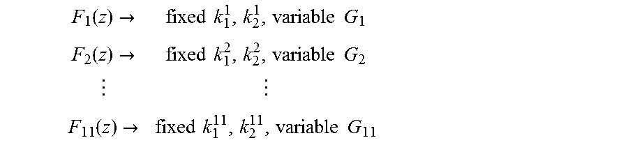
M00011

M00012

M00013

M00014

M00015

M00016

M00017

M00018

M00019

M00020

M00021

M00022

M00023

M00024

M00025

M00026

M00027

M00028

M00029

M00030

M00031

XML
uspto.report is an independent third-party trademark research tool that is not affiliated, endorsed, or sponsored by the United States Patent and Trademark Office (USPTO) or any other governmental organization. The information provided by uspto.report is based on publicly available data at the time of writing and is intended for informational purposes only.
While we strive to provide accurate and up-to-date information, we do not guarantee the accuracy, completeness, reliability, or suitability of the information displayed on this site. The use of this site is at your own risk. Any reliance you place on such information is therefore strictly at your own risk.
All official trademark data, including owner information, should be verified by visiting the official USPTO website at www.uspto.gov. This site is not intended to replace professional legal advice and should not be used as a substitute for consulting with a legal professional who is knowledgeable about trademark law.